Numerical Predictions Using Linear Regression
Predicting sales based on advertising budget—using linear regression in R, Python, and Julia.
Linear regression is important today for making numerical predictions due to its simplicity, interpretability, and effectiveness. By modeling the relationship between a dependent/response/labeled variable and one or more independent/predictor/feature variables, linear regression provides a straightforward framework for estimating values based on known predictors. It allows us to quantify the direction and strength of the relationship, identify important predictors, and make reliable predictions. Linear regression is widely used in various fields, including finance, economics, healthcare, and social sciences, as it provides a practical and intuitive approach to predict numerical outcomes based on the available data and explanatory variables.
Let’s see whether advertising budget offers any ability to predict sales.
Getting Started
If you are interested in reproducing this work, here are the versions of R, Python, and Julia used (as well as the respective packages for each). Additionally, Leland Wilkinson’s approach to data visualization (Grammar of Graphics) has been adopted for this work. Finally, my coding style here is verbose, in order to trace back where functions/methods and variables are originating from, and make this a learning experience for everyone—including me.
cat(
    R.version$version.string, "-", R.version$nickname,
    "\nOS:", Sys.info()["sysname"], R.version$platform,
    "\nCPU:", benchmarkme::get_cpu()$no_of_cores, "x", benchmarkme::get_cpu()$model_name
)
R version 4.2.3 (2023-03-15) - Shortstop Beagle
OS: Darwin x86_64-apple-darwin17.0
CPU: 8 x Intel(R) Core(TM) i5-8259U CPU @ 2.30GHzrequire(devtools)
devtools::install_version("dplyr", version="1.1.4", repos="http://cran.us.r-project.org")
devtools::install_version("ggplot2", version="3.5.0", repos="http://cran.us.r-project.org")
devtools::install_version("caret", version="6.0.94", repos="http://cran.us.r-project.org")library(dplyr)
library(ggplot2)
library(caret)import sys
print(sys.version)3.11.4 (v3.11.4:d2340ef257, Jun 6 2023, 19:15:51) [Clang 13.0.0 (clang-1300.0.29.30)]!pip install pandas==2.0.3
!pip install plotnine==0.12.1
!pip install scikit-learn==1.3.0import random
import datetime
import pandas
import plotnine
import sklearnusing InteractiveUtils
InteractiveUtils.versioninfo()Julia Version 1.9.2
Commit e4ee485e909 (2023-07-05 09:39 UTC)
Platform Info:
OS: macOS (x86_64-apple-darwin22.4.0)
CPU: 8 × Intel(R) Core(TM) i5-8259U CPU @ 2.30GHz
WORD_SIZE: 64
LIBM: libopenlibm
LLVM: libLLVM-14.0.6 (ORCJIT, skylake)
Threads: 1 on 8 virtual cores
Environment:
DYLD_FALLBACK_LIBRARY_PATH = /Library/Frameworks/R.framework/Resources/lib:/Library/Java/JavaVirtualMachines/jdk-21.jdk/Contents/Home/lib/serverusing Pkg
Pkg.add(name="HTTP", version="1.10.2")
Pkg.add(name="CSV", version="0.10.13")
Pkg.add(name="DataFrames", version="1.6.1")
Pkg.add(name="CategoricalArrays", version="0.10.8")
Pkg.add(name="StatsBase", version="0.34.2")
Pkg.add(name="Gadfly", version="1.4.0")using HTTP
using CSV
using DataFrames
using CategoricalArrays
using StatsBase
using GadflyImporting and Examining Dataset
Upon importing and examining the dataset, we can see that the data frame dimension is 200 rows and 5 columns.
advertising_r <- read.csv("https://trevorhastie.github.io/ISLR/Advertising.csv")
str(object=advertising_r)
'data.frame': 200 obs. of 5 variables:
$ X : int 1 2 3 4 5 6 7 8 9 10 ...
$ TV : num 230.1 44.5 17.2 151.5 180.8 ...
$ radio : num 37.8 39.3 45.9 41.3 10.8 48.9 32.8 19.6 2.1 2.6 ...
$ newspaper: num 69.2 45.1 69.3 58.5 58.4 75 23.5 11.6 1 21.2 ...
$ sales : num 22.1 10.4 9.3 18.5 12.9 7.2 11.8 13.2 4.8 10.6 ...head(x=advertising_r, n=8) X TV radio newspaper sales
1 1 230.1 38 69 22.1
2 2 44.5 39 45 10.4
3 3 17.2 46 69 9.3
4 4 151.5 41 58 18.5
5 5 180.8 11 58 12.9
6 6 8.7 49 75 7.2
7 7 57.5 33 24 11.8
8 8 120.2 20 12 13.2tail(x=advertising_r, n=8) X TV radio newspaper sales
193 193 17 4.1 31.6 5.9
194 194 167 42.0 3.6 19.6
195 195 150 35.6 6.0 17.3
196 196 38 3.7 13.8 7.6
197 197 94 4.9 8.1 9.7
198 198 177 9.3 6.4 12.8
199 199 284 42.0 66.2 25.5
200 200 232 8.6 8.7 13.4advertising_py = pandas.read_csv("https://trevorhastie.github.io/ISLR/Advertising.csv")
advertising_py.info()<class 'pandas.core.frame.DataFrame'>
RangeIndex: 200 entries, 0 to 199
Data columns (total 5 columns):
# Column Non-Null Count Dtype
--- ------ -------------- -----
0 Unnamed: 0 200 non-null int64
1 TV 200 non-null float64
2 radio 200 non-null float64
3 newspaper 200 non-null float64
4 sales 200 non-null float64
dtypes: float64(4), int64(1)
memory usage: 7.9 KBadvertising_py.head(n=8) Unnamed: 0 TV radio newspaper sales
0 1 230.1 37.8 69.2 22.1
1 2 44.5 39.3 45.1 10.4
2 3 17.2 45.9 69.3 9.3
3 4 151.5 41.3 58.5 18.5
4 5 180.8 10.8 58.4 12.9
5 6 8.7 48.9 75.0 7.2
6 7 57.5 32.8 23.5 11.8
7 8 120.2 19.6 11.6 13.2advertising_py.tail(n=8) Unnamed: 0 TV radio newspaper sales
192 193 17.2 4.1 31.6 5.9
193 194 166.8 42.0 3.6 19.6
194 195 149.7 35.6 6.0 17.3
195 196 38.2 3.7 13.8 7.6
196 197 94.2 4.9 8.1 9.7
197 198 177.0 9.3 6.4 12.8
198 199 283.6 42.0 66.2 25.5
199 200 232.1 8.6 8.7 13.4advertising_jl = CSV.File(HTTP.get("https://trevorhastie.github.io/ISLR/Advertising.csv").body) |> DataFrames.DataFrame;
describe(advertising_jl)5×7 DataFrame
Row │ variable mean min median max nmissing eltype
│ Symbol Float64 Real Float64 Real Int64 DataType
─────┼───────────────────────────────────────────────────────────────
1 │ Column1 100.5 1 100.5 200 0 Int64
2 │ TV 147.043 0.7 149.75 296.4 0 Float64
3 │ radio 23.264 0.0 22.9 49.6 0 Float64
4 │ newspaper 30.554 0.3 25.75 114.0 0 Float64
5 │ sales 14.0225 1.6 12.9 27.0 0 Float64first(advertising_jl, 8)8×5 DataFrame
Row │ Column1 TV radio newspaper sales
│ Int64 Float64 Float64 Float64 Float64
─────┼───────────────────────────────────────────────
1 │ 1 230.1 37.8 69.2 22.1
2 │ 2 44.5 39.3 45.1 10.4
3 │ 3 17.2 45.9 69.3 9.3
4 │ 4 151.5 41.3 58.5 18.5
5 │ 5 180.8 10.8 58.4 12.9
6 │ 6 8.7 48.9 75.0 7.2
7 │ 7 57.5 32.8 23.5 11.8
8 │ 8 120.2 19.6 11.6 13.2last(advertising_jl, 8)8×5 DataFrame
Row │ Column1 TV radio newspaper sales
│ Int64 Float64 Float64 Float64 Float64
─────┼───────────────────────────────────────────────
1 │ 193 17.2 4.1 31.6 5.9
2 │ 194 166.8 42.0 3.6 19.6
3 │ 195 149.7 35.6 6.0 17.3
4 │ 196 38.2 3.7 13.8 7.6
5 │ 197 94.2 4.9 8.1 9.7
6 │ 198 177.0 9.3 6.4 12.8
7 │ 199 283.6 42.0 66.2 25.5
8 │ 200 232.1 8.6 8.7 13.4Wrangling Data
The first column in the dataset represents the index for each row; it’s extraneous and should be dropped. As an option, to start with simple linear regression (SLR), let’s create a new column that combines all the media budget as a single predictor variable. Lastly, let’s clean-up our data frame by reordering the columns (so that the dependent/response variable is the last column) and forcing the column names to be lowercase.
advertising_clean_r <- advertising_r[, -1]
advertising_clean_r$combined_budget <- advertising_r$TV + advertising_r$radio + advertising_r$newspaper
advertising_clean_r <- advertising_clean_r %>% select(-sales, everything(), sales)
colnames(advertising_clean_r) <- tolower(colnames(advertising_clean_r))
str(object=advertising_clean_r)
'data.frame': 200 obs. of 5 variables:
$ tv : num 230.1 44.5 17.2 151.5 180.8 ...
$ radio : num 37.8 39.3 45.9 41.3 10.8 48.9 32.8 19.6 2.1 2.6 ...
$ newspaper : num 69.2 45.1 69.3 58.5 58.4 75 23.5 11.6 1 21.2 ...
$ combined_budget: num 337 129 132 251 250 ...
$ sales : num 22.1 10.4 9.3 18.5 12.9 7.2 11.8 13.2 4.8 10.6 ...advertising_clean_py = advertising_py.iloc[:, 1:]
advertising_clean_py["combined_budget"] = advertising_clean_py["TV"] + advertising_clean_py["radio"] + advertising_clean_py["newspaper"]
cols = list(advertising_clean_py.columns)
cols.remove('sales')
advertising_clean_py.columns = [col.lower() for col in advertising_clean_py.columns]
advertising_clean_py.info()<class 'pandas.core.frame.DataFrame'>
RangeIndex: 200 entries, 0 to 199
Data columns (total 5 columns):
# Column Non-Null Count Dtype
--- ------ -------------- -----
0 tv 200 non-null float64
1 radio 200 non-null float64
2 newspaper 200 non-null float64
3 sales 200 non-null float64
4 combined_budget 200 non-null float64
dtypes: float64(5)
memory usage: 7.9 KBadvertising_clean_jl = advertising_jl[:, Not(1)];
advertising_clean_jl.combined_budget = advertising_clean_jl.TV + advertising_clean_jl.radio + advertising_clean_jl.newspaper;
advertising_clean_jl = select(advertising_clean_jl, Not(:sales), :sales);
rename!(advertising_clean_jl, lowercase.(names(advertising_clean_jl)));
describe(advertising_clean_jl)5×7 DataFrame
Row │ variable mean min median max nmissing eltype
│ Symbol Float64 Float64 Float64 Float64 Int64 DataType
─────┼──────────────────────────────────────────────────────────────────────────
1 │ tv 147.043 0.7 149.75 296.4 0 Float64
2 │ radio 23.264 0.0 22.9 49.6 0 Float64
3 │ newspaper 30.554 0.3 25.75 114.0 0 Float64
4 │ combined_budget 200.861 11.7 207.35 433.6 0 Float64
5 │ sales 14.0225 1.6 12.9 27.0 0 Float64first(advertising_clean_jl, 8)8×5 DataFrame
Row │ tv radio newspaper combined_budget sales
│ Float64 Float64 Float64 Float64 Float64
─────┼───────────────────────────────────────────────────────
1 │ 230.1 37.8 69.2 337.1 22.1
2 │ 44.5 39.3 45.1 128.9 10.4
3 │ 17.2 45.9 69.3 132.4 9.3
4 │ 151.5 41.3 58.5 251.3 18.5
5 │ 180.8 10.8 58.4 250.0 12.9
6 │ 8.7 48.9 75.0 132.6 7.2
7 │ 57.5 32.8 23.5 113.8 11.8
8 │ 120.2 19.6 11.6 151.4 13.2last(advertising_clean_jl, 8)8×5 DataFrame
Row │ tv radio newspaper combined_budget sales
│ Float64 Float64 Float64 Float64 Float64
─────┼───────────────────────────────────────────────────────
1 │ 17.2 4.1 31.6 52.9 5.9
2 │ 166.8 42.0 3.6 212.4 19.6
3 │ 149.7 35.6 6.0 191.3 17.3
4 │ 38.2 3.7 13.8 55.7 7.6
5 │ 94.2 4.9 8.1 107.2 9.7
6 │ 177.0 9.3 6.4 192.7 12.8
7 │ 283.6 42.0 66.2 391.8 25.5
8 │ 232.1 8.6 8.7 249.4 13.4Performing Exploratory Data Analysis (EDA)
Univariate Analysis
ggplot2::ggplot(advertising_clean_r, aes(x=sales)) +
    geom_histogram()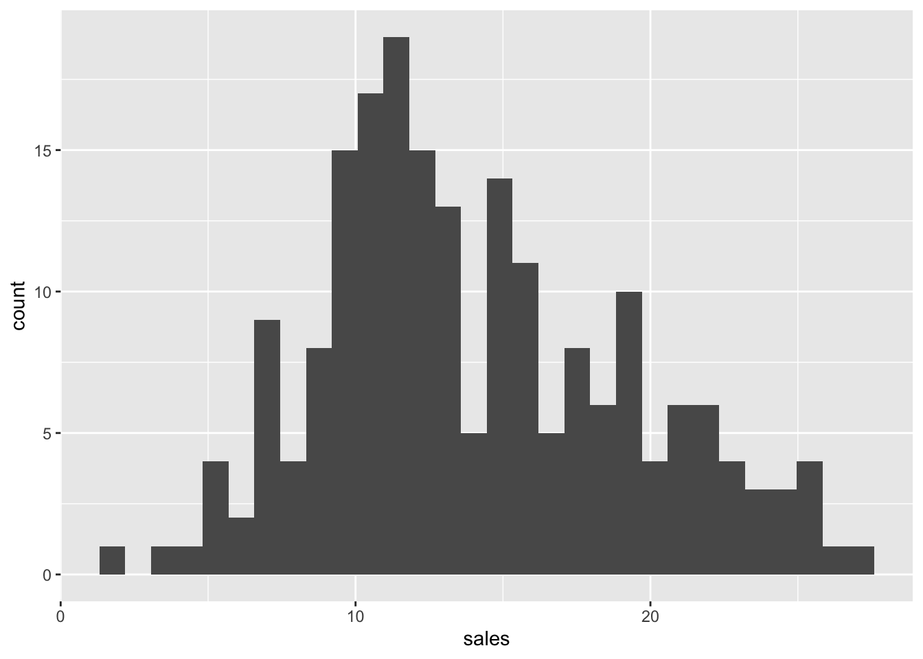
summary(advertising_clean_r$sales) Min. 1st Qu. Median Mean 3rd Qu. Max.
1.6 10.4 12.9 14.0 17.4 27.0 advertising_clean_py.describe() tv radio newspaper sales combined_budget
count 200.000000 200.000000 200.000000 200.000000 200.000000
mean 147.042500 23.264000 30.554000 14.022500 200.860500
std 85.854236 14.846809 21.778621 5.217457 92.985181
min 0.700000 0.000000 0.300000 1.600000 11.700000
25% 74.375000 9.975000 12.750000 10.375000 123.550000
50% 149.750000 22.900000 25.750000 12.900000 207.350000
75% 218.825000 36.525000 45.100000 17.400000 281.125000
max 296.400000 49.600000 114.000000 27.000000 433.600000describe(advertising_clean_jl.sales)Summary Stats:
Length: 200
Missing Count: 0
Mean: 14.022500
Minimum: 1.600000
1st Quartile: 10.375000
Median: 12.900000
3rd Quartile: 17.400000
Maximum: 27.000000
Type: Float64Bivariate Analysis
ggplot2::ggplot(advertising_clean_r, aes(x=combined_budget, y=sales)) +
    geom_point()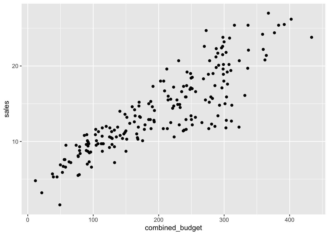
cor(x=advertising_clean_r$combined_budget, y=advertising_clean_r$sales, method="pearson")[1] 0.87ggplot2::ggplot(advertising_clean_r, aes(x=combined_budget, y=tv)) +
geom_point()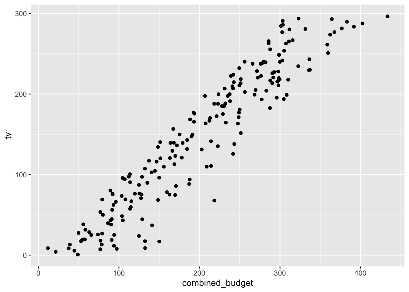
cor(x=advertising_clean_r$tv, y=advertising_clean_r$sales, method="pearson")[1] 0.78ggplot2::ggplot(advertising_clean_r, aes(x=radio, y=sales)) +
geom_point()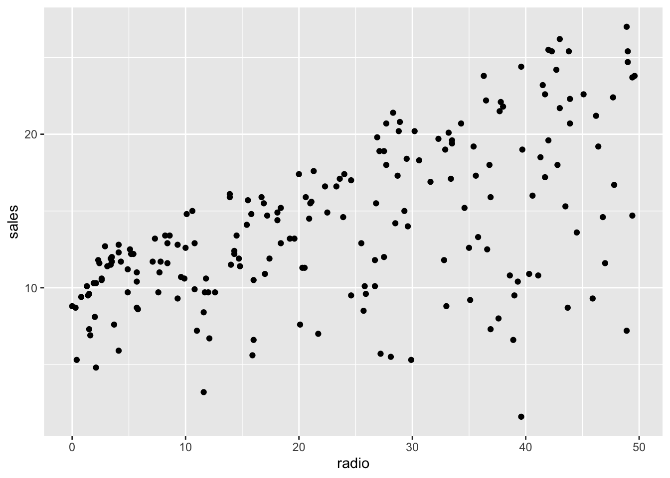
cor(x=advertising_clean_r$radio, y=advertising_clean_r$sales, method="pearson")[1] 0.58ggplot2::ggplot(advertising_clean_r, aes(x=newspaper, y=sales)) +
geom_point()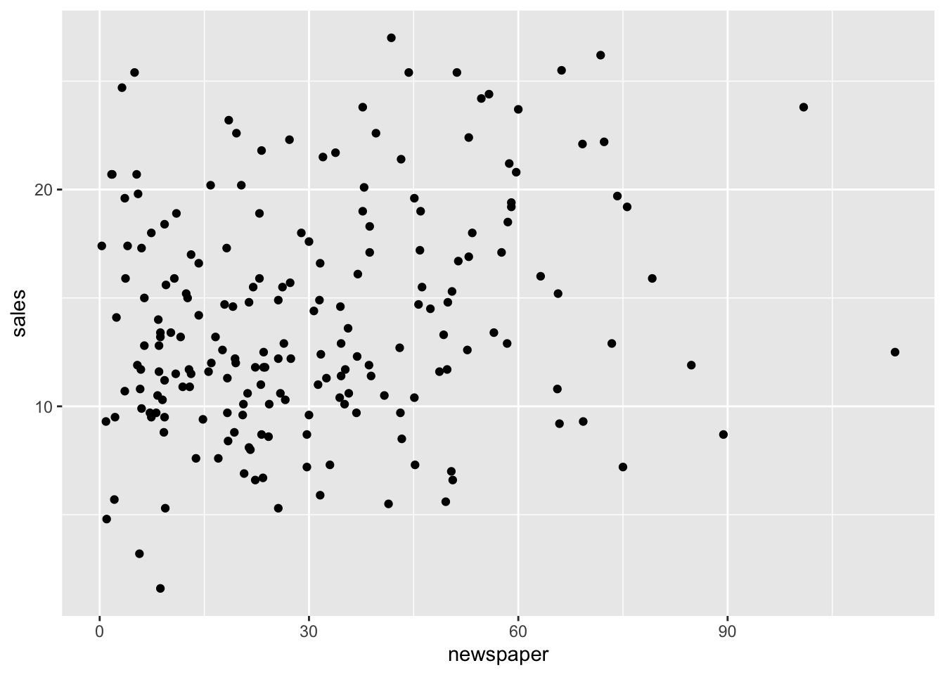
cor(x=advertising_clean_r$newspaper, y=advertising_clean_r$sales, method="pearson")[1] 0.23Splitting Data for Training & Testing
set.seed(1856)
index_train <- createDataPartition(advertising_clean_r$sales, p=0.7, list=FALSE, times=1)
advertising_clean_train_r <- advertising_clean_r[index_train, ]
advertising_clean_test_r <- advertising_clean_r[-index_train, ]
dim(advertising_clean_train_r)
[1] 142 5dim(advertising_clean_test_r)[1] 58 5# walmart_clean_stratified_train_julia,
# walmart_clean_stratified_test_julia = MLJ.partition(
# walmart_clean_jl,
# 0.7,
# rng = 1856,
# stratify = walmart_clean_jl.store
# );
# size(walmart_clean_stratified_train_julia)# histogram_store_train_julia = Gadfly.plot(
# walmart_clean_stratified_train_julia,
# x = "store",
# Gadfly.Geom.histogram(maxbincount = 45),
# Gadfly.Guide.xlabel("Store ID"),
# Gadfly.Guide.ylabel("Count"),
# michaelmallari_theme
# );# size(walmart_clean_stratified_test_julia)
# histogram_store_test_julia = Gadfly.plot(
# walmart_clean_stratified_test_julia,
# x = "store",
# Gadfly.Geom.histogram(maxbincount = 45),
# Gadfly.Guide.xlabel("Store ID"),
# Gadfly.Guide.ylabel("Count"),
# michaelmallari_theme
# );Fitting For Linear Model (Simple Linear Regression)
slr_fit_r <- lm(
    formula=sales ~ combined_budget,
    data=advertising_clean_train_r
)
summary(slr_fit_r)
Call:
lm(formula = sales ~ combined_budget, data = advertising_clean_train_r)

Residuals:
   Min     1Q Median     3Q    Max
-7.165 -1.444  0.073  1.691  7.213

Coefficients:
                Estimate Std. Error t value             Pr(>|t|)
(Intercept)      4.14858    0.50920    8.15     0.00000000000019 ***
combined_budget  0.04895    0.00228   21.48 < 0.0000000000000002 ***
---
Signif. codes:  0 '***' 0.001 '**' 0.01 '*' 0.05 '.' 0.1 ' ' 1

Residual standard error: 2.5 on 140 degrees of freedom
Multiple R-squared:  0.767,	Adjusted R-squared:  0.766
F-statistic: 462 on 1 and 140 DF, p-value: <0.0000000000000002slr_fit_julia = lm(
@formula(sales ~ combined_budget,
advertising_clean_julia
)Fitting For Linear Model (Multiple Linear Regression)
mlr_fit_r <- lm(
    formula=sales ~ tv + radio + newspaper,
    data=advertising_clean_train_r
)
summary(mlr_fit_r)
Call:
lm(formula = sales ~ tv + radio + newspaper, data = advertising_clean_train_r)

Residuals:
   Min     1Q Median     3Q    Max
-5.101 -0.935  0.200  1.160  2.823

Coefficients:
            Estimate Std. Error t value             Pr(>|t|)
(Intercept)  2.97682    0.35515    8.38    0.000000000000054 ***
tv           0.04600    0.00153   30.02 < 0.0000000000000002 ***
radio        0.18931    0.00982   19.28 < 0.0000000000000002 ***
newspaper   -0.00445    0.00639   -0.70                 0.49
---
Signif. codes:  0 '***' 0.001 '**' 0.01 '*' 0.05 '.' 0.1 ' ' 1

Residual standard error: 1.6 on 138 degrees of freedom
Multiple R-squared:  0.909,	Adjusted R-squared:  0.908
F-statistic: 462 on 3 and 138 DF, p-value: <0.0000000000000002Making Predictions With Test Data
Evaluating Model Predictions
Further Readings
- Hildebrand, D. K., Ott, R. L., & Gray, J. B. (2005). Basic Statistical Ideas for Managers (2nd ed.). Thompson Brooks/Cole.
- James, G., Witten, D., Hastie, T., & Tibshirani, R. (2021). An Introduction to Statistical Learning: With Applications in R (2nd ed.). Springer. https://doi.org/10.1007/978-1-0716-1418-1
- Kuhn, M. & Johnson, K. (2013). Applied Predictive Modeling. Springer. https://doi.org/10.1007/978-1-4614-6849-3
- Stine, R. & Foster, D. (2017). Statistics for Business: Decision Making and Anlysis (3rd ed.). Pearson.