Covariance and Correlation
Analyzing the linear predictive strength of the factors that makes a great wine—using R, Python, and Julia.
Covariance and correlation are useful in understanding wine as they provide insights into the relationships between different wine attributes. Covariance measures the direction and strength of the linear relationship between two variables, such as the correlation between wine price and quality. Correlation, on the other hand, provides a standardized measure of the strength and direction of the linear relationship between variables, such as the correlation between wine acidity and perceived freshness. By analyzing covariance and correlation, we can identify patterns, understand the impact of variables on wine characteristics, and make informed decisions in areas like grape selection, winemaking processes, and consumer preferences. Let’s see these concepts in action.
Getting Started
If you are interested in reproducing this work, here are the versions of R, Python, and Julia used (as well as the respective packages for each). Additionally, my coding style here is verbose, in order to trace back where functions/methods and variables are originating from, and make this a learning experience for everyone—including me.
cat(R.version$version.string, R.version$nickname)R version 4.2.3 (2023-03-15) Shortstop Beaglerequire(devtools)
devtools::install_version("dplyr", version="1.1.2", repos="http://cran.us.r-project.org")
devtools::install_version("ggplot2", version="3.4.2", repos="http://cran.us.r-project.org")
devtools::install_version("corrplot", version="0.92", repos="http://cran.us.r-project.org")library(dplyr)
library(ggplot2)
library(corrplot)import sys
print(sys.version)3.11.4 (v3.11.4:d2340ef257, Jun 6 2023, 19:15:51) [Clang 13.0.0 (clang-1300.0.29.30)]!pip install pyreadr==0.4.7
!pip install numpy==1.25.1
!pip install pandas==2.0.3
!pip install plotnine==0.12.1
!pip install scipy==1.11.1import pyreadr
import numpy
import pandas
import plotnine
from scipy import statsusing InteractiveUtils
InteractiveUtils.versioninfo()Julia Version 1.9.2
Commit e4ee485e909 (2023-07-05 09:39 UTC)
Platform Info:
OS: macOS (x86_64-apple-darwin22.4.0)
CPU: 8 × Intel(R) Core(TM) i5-8259U CPU @ 2.30GHz
WORD_SIZE: 64
LIBM: libopenlibm
LLVM: libLLVM-14.0.6 (ORCJIT, skylake)
Threads: 1 on 8 virtual cores
Environment:
DYLD_FALLBACK_LIBRARY_PATH = /Library/Frameworks/R.framework/Resources/lib:/Library/Java/JavaVirtualMachines/jdk1.8.0_241.jdk/Contents/Home/jre/lib/serverusing Pkg
Pkg.add(name="RData", version="0.8.3")
Pkg.add(name="CSV", version="0.10.11")
Pkg.add(name="DataFrames", version="1.5.0")
Pkg.add(name="CategoricalArrays", version="0.10.8")
Pkg.add(name="Colors", version="0.12.10")
Pkg.add(name="Cairo", version="1.0.5")
Pkg.add(name="Gadfly", version="1.3.4")
Pkg.add(name="StatsBase", version="0.33.21")using RData
using CSV
using DataFrames
using CategoricalArrays
using Colors
using Cairo
using Gadfly
using StatsBaseImporting Data
wine_quality_red <- read.csv("http://archive.ics.uci.edu/ml/machine-learning-databases/wine-quality/winequality-red.csv", sep = ";")
wine_quality_white <- read.csv("http://archive.ics.uci.edu/ml/machine-learning-databases/wine-quality/winequality-white.csv", sep = ";")
wine_quality_red$type <- as.factor("red")
wine_quality_white$type <- as.factor("white")wine_quality <- rbind(wine_quality_red, wine_quality_white)
str(wine_quality)'data.frame': 6497 obs. of 13 variables:
$ fixed_acidity : num 7.4 7.8 7.8 11.2 7.4 7.4 7.9 7.3 7.8 7.5 ...
$ volatile_acidity : num 0.7 0.88 0.76 0.28 0.7 0.66 0.6 0.65 0.58 0.5 ...
$ citric_acid : num 0 0 0.04 0.56 0 0 0.06 0 0.02 0.36 ...
$ residual_sugar : num 1.9 2.6 2.3 1.9 1.9 1.8 1.6 1.2 2 6.1 ...
$ chlorides : num 0.076 0.098 0.092 0.075 0.076 0.075 0.069 0.065 0.073 0.071 ...
$ free_sulfur_dioxide : num 11 25 15 17 11 13 15 15 9 17 ...
$ total_sulfur_dioxide: num 34 67 54 60 34 40 59 21 18 102 ...
$ density : num 0.998 0.997 0.997 0.998 0.998 ...
$ pH : num 3.51 3.2 3.26 3.16 3.51 3.51 3.3 3.39 3.36 3.35 ...
$ sulphates : num 0.56 0.68 0.65 0.58 0.56 0.56 0.46 0.47 0.57 0.8 ...
$ alcohol : num 9.4 9.8 9.8 9.8 9.4 9.4 9.4 10 9.5 10.5 ...
$ quality : int 5 5 5 6 5 5 5 7 7 5 ...
$ type : Factor w/ 2 levels "red","white": 1 1 1 1 1 1 1 1 1 1 ...Covariance
wine_quality_cov = cov(wine_quality[1:12])round(wine_quality_cov, 2) fixed_acidity volatile_acidity citric_acid residual_sugar chlorides free_sulfur_dioxide total_sulfur_dioxide density pH sulphates alcohol quality
fixed_acidity 1.68 0.05 0.06 -0.69 0.01 -6.51 -24.11 0.00 -0.05 0.06 -0.15 -0.09
volatile_acidity 0.05 0.03 -0.01 -0.15 0.00 -1.03 -3.86 0.00 0.01 0.01 -0.01 -0.04
citric_acid 0.06 -0.01 0.02 0.10 0.00 0.34 1.60 0.00 -0.01 0.00 0.00 0.01
residual_sugar -0.69 -0.15 0.10 22.64 -0.02 34.02 133.24 0.01 -0.20 -0.13 -2.04 -0.15
chlorides 0.01 0.00 0.00 -0.02 0.00 -0.12 -0.55 0.00 0.00 0.00 -0.01 -0.01
free_sulfur_dioxide -6.51 -1.03 0.34 34.02 -0.12 315.04 723.26 0.00 -0.42 -0.50 -3.81 0.86
total_sulfur_dioxide -24.11 -3.86 1.60 133.24 -0.55 723.26 3194.72 0.01 -2.17 -2.32 -17.91 -2.04
density 0.00 0.00 0.00 0.01 0.00 0.00 0.01 0.00 0.00 0.00 0.00 0.00
pH -0.05 0.01 -0.01 -0.20 0.00 -0.42 -2.17 0.00 0.03 0.00 0.02 0.00
sulphates 0.06 0.01 0.00 -0.13 0.00 -0.50 -2.32 0.00 0.00 0.02 0.00 0.01
alcohol -0.15 -0.01 0.00 -2.04 -0.01 -3.81 -17.91 0.00 0.02 0.00 1.42 0.46
quality -0.09 -0.04 0.01 -0.15 -0.01 0.86 -2.04 0.00 0.00 0.01 0.46 0.76Correlation
There are three main methods to measure correlation: Pearson’s r, Kendall’s τ (tau), and Spearman’s ρ (rho). Pearson’s r is the most commonly used method, as it essentially normalizes the range of covariance to +1 and -1. Let’s visualize the correlation within the dataset.
wine_quality_cor_pearson = cor(wine_quality[1:12], method = "pearson")
correlation_matrix <- as.data.frame(wine_quality_cor_pearson)
correlation_matrix$var1 <- rownames(correlation_matrix)
correlation_matrix %>%
    tidyr::gather(key = var2, value = r, 1:12) %>%
    ggplot2::ggplot(aes(x = var1, y = var2, fill = r)) +
    ggplot2::geom_tile() +
    ggplot2::geom_text(aes(label = round(r, 2)), size = 2.2) +
    ggplot2::scale_fill_gradient2(low = "#eb3300", high = "#00a6c8", mid = "white") +
    ggplot2::labs(title = "Correlation Matrix for Red and White Wines", subtitle = "Pearson's Correlation Coefficient (r)", x = "", y = "") +
    ggplot2::theme(axis.text.x = element_text(angle = 45, hjust = 1), plot.title = element_text(size = 16, face = "bold", hjust = 0.5), plot.subtitle = element_text(size = 12, hjust = 0.5))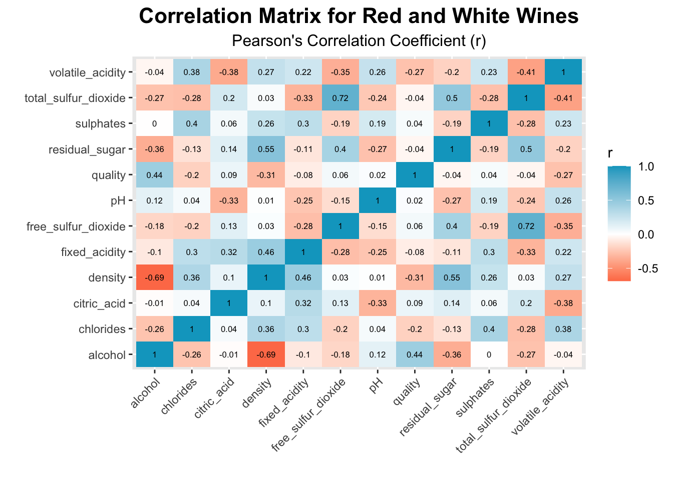
What Correlates with Quality
The quality score (our dependent variable) is based on a ranking between 1 and 10. Based on the Pearson’s correlation coefficient (r), three independent variables demonstrate meaningful direction and strength:
- Alcohol (+0.44)
- Density (-0.31)
- Volatile Acidity (-0.27)
Given that the initial correlation matrix combines the red wine and white wine dataset, let’s now see what happens when we visual the correlation matrix separately for the two wine types.
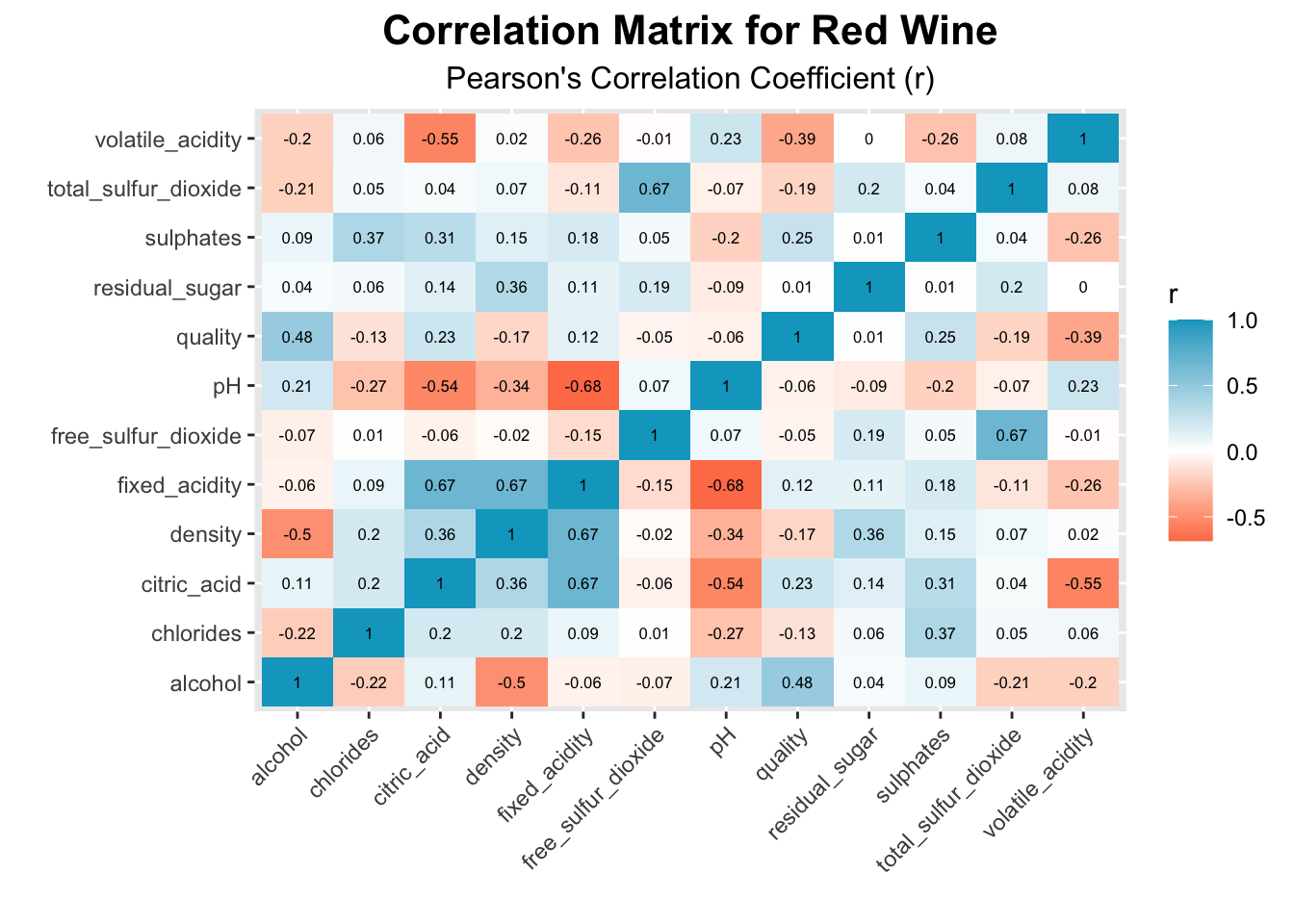
We can see that the quality of red wine is mainly attributed to four variables:
- Alcohol (+0.48)
- Volatile Acidity (-0.39)
- Sulphates (+0.25)
- Citric Acid (+0.23)
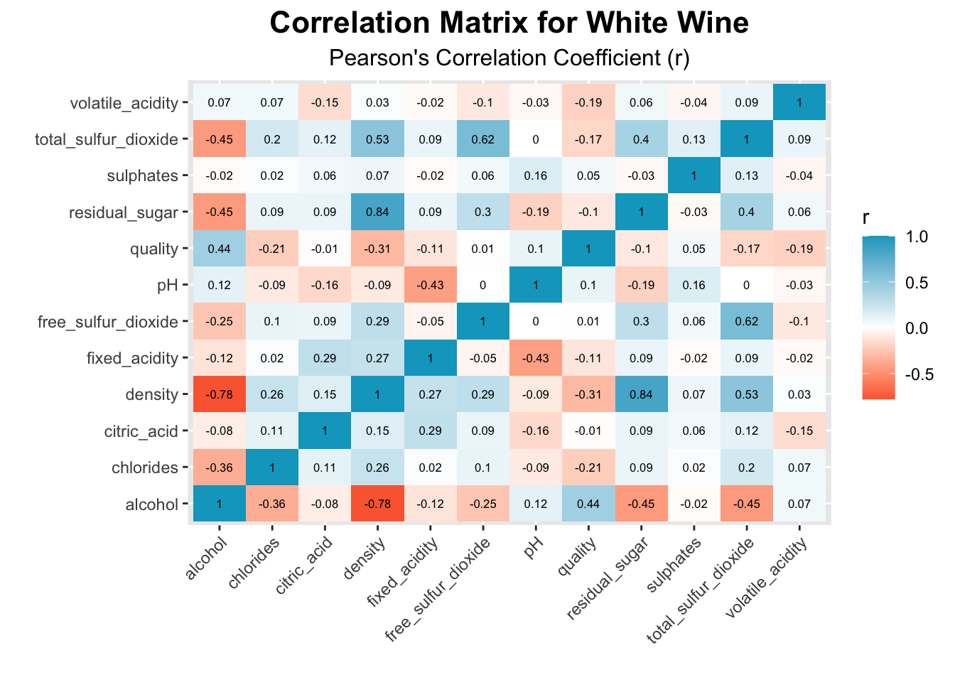
Meanwhile, the quality of white wine is mainly attributed to three variables:
- Alcohol (+0.44)
- Density (-0.31)
- Chlorides (-0.21)
A Precursor to Linear Regression
Before you can apply linear regression techniques to create a predictive model for the quality of your home-made wine, you must first satisfy the linear relationship requirements in order to properly use those techniques. Calculating the correlation in your dataset is one way to determine the linear relationships in your data.