Data Types and Data Structures
Understanding the NHANES data types and data structures—one of the first steps of any data analysis—using Julia, Python, and R.
Let’s face it… there is an abundance of data being generated every second, but we are yet to truly unlock its full potential. The very first step in doing so is understanding data at its atomic level; what is it (data type) and how is it stored and accessed (data structures)? For this post, I’ll focus on commonly used data types and data structures in data science (a subset of computer science).
Getting Started
If you are interested in reproducing this work, here are the versions of Julia, Python, and R used (as well as the respective packages for each). In addition, Leland Wilkinson’s approach to data visualization (Grammar of Graphics) has been adopted in this work.
VERSIONv"1.5.0"import Pkg
Pkg.add(name="CSV", version="0.10.4")
Pkg.add(name="DataFrames", version="1.5.0")
Pkg.add(name="CategoricalArrays", version="0.10.7")
Pkg.add(name="StatsBase", version="0.33.21")
Pkg.add(name="Colors", version="0.12.10")
Pkg.add(name="Cairo", version="1.0.5")
Pkg.add(name="Gadfly", version="1.3.4")using CSV
using DataFrames
using CategoricalArrays
using StatsBase
using Colors
using Cairo
using Gadflyimport sys
print(sys.version)3.9.6 (v3.9.6:db3ff76da1, Jun 28 2021, 11:49:53)
[Clang 6.0 (clang-600.0.57)]!pip install pandas==2.0.0
!pip install plotnine==0.10.1import pandas
import plotnineR.version.string[1] "R version 4.1.1 (2021-08-10)"require(devtools)
devtools::install_version("dplyr", version="1.0.10", repos="http://cran.us.r-project.org")
devtools::install_version("ggplot2", version="3.4.0", repos="http://cran.us.r-project.org")
devtools::install_version("epiDisplay", version="3.5.0.2", repos="http://cran.us.r-project.org")library(dplyr)
library(ggplot2)
library(epiDisplay)Importing and Examining Dataset
The U.S. National Health and Nutrition Examination Study (NHANES) has made its 1999-2004 data available. After importing this data, we then look into the data structure (and data types stored in it), in order to determine whether data preparation is needed. In real life, 80% of a data analyst’s time is spent on data preparation (also known as data wrangling). Note: I’ve already done some data preparation. The data below will look slightly different than yours.
nhanes_jl = CSV.File("../../dataset/nhanes.csv") |> DataFrames.DataFrame10000×76 DataFrame
Row │ id survey_year gender age age_decade age_months race_1 race_3 education marital_status hh_income hh_income_mid poverty home_rooms home_own work weight length head_circ height bmi bmi_cat_under_20yrs bmi_who pulse bp_sys_ave bp_dia_ave bp_sys_1 BPDia1 bp_sys_2 bp_dia_2 bp_sys_3 BPDia3 Testosterone DirectChol TotChol UrineVol1 UrineFlow1 UrineVol2 UrineFlow2 diabetes DiabetesAge health_gen DaysPhysHlthBad DaysMentHlthBad little_interest depressed nPregnancies nBabies Age1stBaby SleepHrsNight sleep_trouble phys_active PhysActiveDays tv_hrs_day comp_hrs_day TVHrsDayChild CompHrsDayChild alcohol_12_plus_yr AlcoholDay alcohol_year smoke_now smoke_100 smoke_100n smoke_age marijuana age_first_marij regular_marij age_reg_marij hard_drugs sex_ever sex_age sex_num_partn_life sex_num_part_year same_sex sex_orientation pregnant_now
│ Int64 String7 String7 Int64 String7? Int64? String15 String15? String15? String15? String15? Int64? Float64? Int64? String7? String15? Float64? Float64? Float64? Float64? Float64? String15? String15? Int64? Int64? Int64? Int64? Int64? Int64? Int64? Int64? Int64? Float64? Float64? Float64? Int64? Float64? Int64? Float64? String3? Int64? String15? Int64? Int64? String7? String7? Int64? Int64? Int64? Int64? String3? String3? Int64? String15? String15? Int64? Int64? String3? Int64? Int64? String3? String3? String15? Int64? String3? Int64? String3? Int64? String3? String3? Int64? Int64? Int64? String3? String15? String7
───────┼─────────────────────────────────────────────────────────────────────────────────────────────────────────────────────────────────────────────────────────────────────────────────────────────────────────────────────────────────────────────────────────────────────────────────────────────────────────────────────────────────────────────────────────────────────────────────────────────────────────────────────────────────────────────────────────────────────────────────────────────────────────────────────────────────────────────────────────────────────────────────────────────────────────────────────────────────────────────────────────────────────────────────────────────────────────────────────────────────────────────────────────────────────────────────────────────────────────────────────────────────────────────────────────────────────────────────────────────────────────────────────────────────────────────────────────────────────────────────────────────────
1 │ 51624 2009_10 male 34 30-39 409 White missing High School Married 25000-34999 30000 1.36 6 Own NotWorking 87.4 missing missing 164.7 32.22 missing 30.0_plus 70 113 85 114 88 114 88 112 82 missing 1.29 3.49 352 missing missing missing No missing Good 0 15 Most Several missing missing missing 4 Yes No missing missing missing missing missing Yes missing 0 No Yes Smoker 18 Yes 17 No missing Yes Yes 16 8 1 No Heterosexual
2 │ 51624 2009_10 male 34 30-39 409 White missing High School Married 25000-34999 30000 1.36 6 Own NotWorking 87.4 missing missing 164.7 32.22 missing 30.0_plus 70 113 85 114 88 114 88 112 82 missing 1.29 3.49 352 missing missing missing No missing Good 0 15 Most Several missing missing missing 4 Yes No missing missing missing missing missing Yes missing 0 No Yes Smoker 18 Yes 17 No missing Yes Yes 16 8 1 No Heterosexual
3 │ 51624 2009_10 male 34 30-39 409 White missing High School Married 25000-34999 30000 1.36 6 Own NotWorking 87.4 missing missing 164.7 32.22 missing 30.0_plus 70 113 85 114 88 114 88 112 82 missing 1.29 3.49 352 missing missing missing No missing Good 0 15 Most Several missing missing missing 4 Yes No missing missing missing missing missing Yes missing 0 No Yes Smoker 18 Yes 17 No missing Yes Yes 16 8 1 No Heterosexual
4 │ 51625 2009_10 male 4 0-9 49 Other missing missing missing 20000-24999 22500 1.07 9 Own missing 17.0 missing missing 105.4 15.3 missing 12.0_18.5 missing missing missing missing missing missing missing missing missing missing missing missing missing missing missing missing No missing missing missing missing missing missing missing missing missing missing missing missing missing missing missing 4 1 missing missing missing missing missing missing missing missing missing missing missing missing missing missing missing missing missing missing
5 │ 51630 2009_10 female 49 40-49 596 White missing Some College LivePartner 35000-44999 40000 1.91 5 Rent NotWorking 86.7 missing missing 168.4 30.57 missing 30.0_plus 86 112 75 118 82 108 74 116 76 missing 1.16 6.7 77 0.094 missing missing No missing Good 0 10 Several Several 2 2 27 8 Yes No missing missing missing missing missing Yes 2 20 Yes Yes Smoker 38 Yes 18 No missing Yes Yes 12 10 1 Yes Heterosexual
6 │ 51638 2009_10 male 9 0-9 115 White missing missing missing 75000-99999 87500 1.84 6 Rent missing 29.8 missing missing 133.1 16.82 missing 12.0_18.5 82 86 47 84 50 84 50 88 44 missing 1.34 4.86 123 1.538 missing missing No missing missing missing missing missing missing missing missing missing missing missing missing missing missing missing 5 0 missing missing missing missing missing missing missing missing missing missing missing missing missing missing missing missing missing missing
7 │ 51646 2009_10 male 8 0-9 101 White missing missing missing 55000-64999 60000 2.33 7 Own missing 35.2 missing missing 130.6 20.64 missing 18.5_to_24.9 72 107 37 114 46 108 36 106 38 missing 1.55 4.09 238 1.322 missing missing No missing missing missing missing missing missing missing missing missing missing missing missing missing missing missing 1 6 missing missing missing missing missing missing missing missing missing missing missing missing missing missing missing missing missing missing
8 │ 51647 2009_10 female 45 40-49 541 White missing College Grad Married 75000-99999 87500 5.0 6 Own Working 75.7 missing missing 166.7 27.24 missing 25.0_to_29.9 62 118 64 106 62 118 68 118 60 missing 2.12 5.82 106 1.116 missing missing No missing Vgood 0 3 None None 1 missing missing 8 No Yes 5 missing missing missing missing Yes 3 52 missing No Non-Smoker missing Yes 13 No missing No Yes 13 20 0 Yes Bisexual
⋮ │ ⋮ ⋮ ⋮ ⋮ ⋮ ⋮ ⋮ ⋮ ⋮ ⋮ ⋮ ⋮ ⋮ ⋮ ⋮ ⋮ ⋮ ⋮ ⋮ ⋮ ⋮ ⋮ ⋮ ⋮ ⋮ ⋮ ⋮ ⋮ ⋮ ⋮ ⋮ ⋮ ⋮ ⋮ ⋮ ⋮ ⋮ ⋮ ⋮ ⋮ ⋮ ⋮ ⋮ ⋮ ⋮ ⋮ ⋮ ⋮ ⋮ ⋮ ⋮ ⋮ ⋮ ⋮ ⋮ ⋮ ⋮ ⋮ ⋮ ⋮ ⋮ ⋮ ⋮ ⋮ ⋮ ⋮ ⋮ ⋮ ⋮ ⋮ ⋮ ⋮ ⋮ ⋮ ⋮ ⋮
9994 │ 71909 2011_12 male 28 20-29 missing Mexican Mexican 9 - 11th Grade NeverMarried 5000-9999 7500 0.46 3 Rent Working 92.3 missing missing 177.3 29.4 missing 25.0_to_29.9 68 124 65 124 62 126 64 122 66 490.43 1.22 3.9 97 0.942 missing missing No missing missing missing missing missing missing missing missing missing 6 No Yes missing 1_hr 2_hr missing missing missing missing missing Yes Yes Smoker 18 missing missing missing missing missing missing missing missing missing missing missing
9995 │ 71909 2011_12 male 28 20-29 missing Mexican Mexican 9 - 11th Grade NeverMarried 5000-9999 7500 0.46 3 Rent Working 92.3 missing missing 177.3 29.4 missing 25.0_to_29.9 68 124 65 124 62 126 64 122 66 490.43 1.22 3.9 97 0.942 missing missing No missing missing missing missing missing missing missing missing missing 6 No Yes missing 1_hr 2_hr missing missing missing missing missing Yes Yes Smoker 18 missing missing missing missing missing missing missing missing missing missing missing
9996 │ 71909 2011_12 male 28 20-29 missing Mexican Mexican 9 - 11th Grade NeverMarried 5000-9999 7500 0.46 3 Rent Working 92.3 missing missing 177.3 29.4 missing 25.0_to_29.9 68 124 65 124 62 126 64 122 66 490.43 1.22 3.9 97 0.942 missing missing No missing missing missing missing missing missing missing missing missing 6 No Yes missing 1_hr 2_hr missing missing missing missing missing Yes Yes Smoker 18 missing missing missing missing missing missing missing missing missing missing missing
9997 │ 71910 2011_12 female 0 0-9 5 White White missing missing 75000-99999 87500 3.37 10 Own missing 6.7 67.6 42.2 missing missing missing missing missing missing missing missing missing missing missing missing missing missing missing missing missing missing missing missing missing missing missing missing missing missing missing missing missing missing missing missing missing missing missing missing missing missing missing missing missing missing missing missing missing missing missing missing missing missing missing missing missing missing missing missing
9998 │ 71911 2011_12 male 27 20-29 missing Mexican Mexican College Grad Married 75000-99999 87500 3.25 10 Own Working 96.7 missing missing 175.8 31.3 missing 30.0_plus 74 133 74 122 76 132 82 134 66 509.0 1.06 5.72 63 0.6 missing missing No missing Good 0 2 None None missing missing missing 6 No No 3 1_hr 0_to_1_hr missing missing Yes 5 4 missing No Non-Smoker missing Yes 22 No missing No Yes 21 1 1 No Heterosexual
9999 │ 71915 2011_12 male 60 60-69 missing White White College Grad NeverMarried 65000-74999 70000 5.0 4 Own Working 78.4 missing missing 168.8 27.5 missing 25.0_to_29.9 76 147 73 150 72 148 74 146 72 505.13 0.93 4.94 218 1.253 missing missing Yes 56 Good 0 2 None None missing missing missing 6 No No 1 2_hr 1_hr missing missing Yes missing 0 missing No Non-Smoker missing missing missing missing missing No Yes 19 2 missing No missing
10000 │ 71915 2011_12 male 60 60-69 missing White White College Grad NeverMarried 65000-74999 70000 5.0 4 Own Working 78.4 missing missing 168.8 27.5 missing 25.0_to_29.9 76 147 73 150 72 148 74 146 72 505.13 0.93 4.94 218 1.253 missing missing Yes 56 Good 0 2 None None missing missing missing 6 No No missing 2_hr 1_hr missing missing Yes missing 0 missing No Non-Smoker missing missing missing missing missing No Yes 19 2 missing No missing
9985 rows omittednhanes_py = pandas.read_csv("../../dataset/nhanes.csv")
nhanes_py.info()<class 'pandas.core.frame.DataFrame'>
RangeIndex: 10000 entries, 0 to 9999
Data columns (total 76 columns):
# Column Non-Null Count Dtype
--- ------ -------------- -----
0 id 10000 non-null int64
1 survey_year 10000 non-null object
2 gender 10000 non-null object
3 age 10000 non-null int64
4 age_decade 9667 non-null object
5 age_months 4962 non-null float64
6 race_1 10000 non-null object
7 race_3 5000 non-null object
8 education 7221 non-null object
9 marital_status 7231 non-null object
10 hh_income 9189 non-null object
11 hh_income_mid 9189 non-null float64
12 poverty 9274 non-null float64
13 home_rooms 9931 non-null float64
14 home_own 9937 non-null object
15 work 7771 non-null object
16 weight 9922 non-null float64
17 length 543 non-null float64
18 head_circ 88 non-null float64
19 height 9647 non-null float64
20 bmi 9634 non-null float64
21 bmi_cat_under_20yrs 1274 non-null object
22 bmi_who 9603 non-null object
23 pulse 8563 non-null float64
24 bp_sys_ave 8551 non-null float64
25 bp_dia_ave 8551 non-null float64
26 bp_sys_1 8237 non-null float64
27 BPDia1 8237 non-null float64
28 bp_sys_2 8353 non-null float64
29 bp_dia_2 8353 non-null float64
30 bp_sys_3 8365 non-null float64
31 BPDia3 8365 non-null float64
32 Testosterone 4126 non-null float64
33 DirectChol 8474 non-null float64
34 TotChol 8474 non-null float64
35 UrineVol1 9013 non-null float64
36 UrineFlow1 8397 non-null float64
37 UrineVol2 1478 non-null float64
38 UrineFlow2 1476 non-null float64
39 diabetes 9858 non-null object
40 DiabetesAge 629 non-null float64
41 health_gen 7539 non-null object
42 DaysPhysHlthBad 7532 non-null float64
43 DaysMentHlthBad 7534 non-null float64
44 little_interest 1564 non-null object
45 depressed 1427 non-null object
46 nPregnancies 2604 non-null float64
47 nBabies 2416 non-null float64
48 Age1stBaby 1884 non-null float64
49 SleepHrsNight 7755 non-null float64
50 sleep_trouble 7772 non-null object
51 phys_active 8326 non-null object
52 PhysActiveDays 4663 non-null float64
53 tv_hrs_day 4859 non-null object
54 comp_hrs_day 4863 non-null object
55 TVHrsDayChild 653 non-null float64
56 CompHrsDayChild 653 non-null float64
57 alcohol_12_plus_yr 6580 non-null object
58 AlcoholDay 4914 non-null float64
59 alcohol_year 5922 non-null float64
60 smoke_now 3211 non-null object
61 smoke_100 7235 non-null object
62 smoke_100n 7235 non-null object
63 smoke_age 3080 non-null float64
64 marijuana 4941 non-null object
65 age_first_marij 2891 non-null float64
66 regular_marij 4941 non-null object
67 age_reg_marij 1366 non-null float64
68 hard_drugs 5765 non-null object
69 sex_ever 5767 non-null object
70 sex_age 5540 non-null float64
71 sex_num_partn_life 5725 non-null float64
72 sex_num_part_year 4928 non-null float64
73 same_sex 5768 non-null object
74 sex_orientation 4842 non-null object
75 pregnant_now 10000 non-null object
dtypes: float64(43), int64(2), object(31)
memory usage: 5.8+ MBnhanes_py.head(n=8) id survey_year gender age age_decade age_months race_1 race_3 education marital_status hh_income hh_income_mid poverty home_rooms home_own work weight length head_circ height bmi bmi_cat_under_20yrs bmi_who pulse bp_sys_ave bp_dia_ave bp_sys_1 BPDia1 bp_sys_2 bp_dia_2 bp_sys_3 BPDia3 Testosterone DirectChol TotChol UrineVol1 UrineFlow1 UrineVol2 UrineFlow2 diabetes DiabetesAge health_gen DaysPhysHlthBad DaysMentHlthBad little_interest depressed nPregnancies nBabies Age1stBaby SleepHrsNight sleep_trouble phys_active PhysActiveDays tv_hrs_day comp_hrs_day TVHrsDayChild CompHrsDayChild alcohol_12_plus_yr AlcoholDay alcohol_year smoke_now smoke_100 smoke_100n smoke_age marijuana age_first_marij regular_marij age_reg_marij hard_drugs sex_ever sex_age sex_num_partn_life sex_num_part_year same_sex sex_orientation pregnant_now
0 51624 2009_10 male 34 30-39 409.0 White NaN High School Married 25000-34999 30000.0 1.36 6.0 Own NotWorking 87.4 NaN NaN 164.7 32.22 NaN 30.0_plus 70.0 113.0 85.0 114.0 88.0 114.0 88.0 112.0 82.0 NaN 1.29 3.49 352.0 NaN NaN NaN No NaN Good 0.0 15.0 Most Several NaN NaN NaN 4.0 Yes No NaN NaN NaN NaN NaN Yes NaN 0.0 No Yes Smoker 18.0 Yes 17.0 No NaN Yes Yes 16.0 8.0 1.0 No Heterosexual
1 51624 2009_10 male 34 30-39 409.0 White NaN High School Married 25000-34999 30000.0 1.36 6.0 Own NotWorking 87.4 NaN NaN 164.7 32.22 NaN 30.0_plus 70.0 113.0 85.0 114.0 88.0 114.0 88.0 112.0 82.0 NaN 1.29 3.49 352.0 NaN NaN NaN No NaN Good 0.0 15.0 Most Several NaN NaN NaN 4.0 Yes No NaN NaN NaN NaN NaN Yes NaN 0.0 No Yes Smoker 18.0 Yes 17.0 No NaN Yes Yes 16.0 8.0 1.0 No Heterosexual
2 51624 2009_10 male 34 30-39 409.0 White NaN High School Married 25000-34999 30000.0 1.36 6.0 Own NotWorking 87.4 NaN NaN 164.7 32.22 NaN 30.0_plus 70.0 113.0 85.0 114.0 88.0 114.0 88.0 112.0 82.0 NaN 1.29 3.49 352.0 NaN NaN NaN No NaN Good 0.0 15.0 Most Several NaN NaN NaN 4.0 Yes No NaN NaN NaN NaN NaN Yes NaN 0.0 No Yes Smoker 18.0 Yes 17.0 No NaN Yes Yes 16.0 8.0 1.0 No Heterosexual
3 51625 2009_10 male 4 0-9 49.0 Other NaN NaN NaN 20000-24999 22500.0 1.07 9.0 Own NaN 17.0 NaN NaN 105.4 15.30 NaN 12.0_18.5 NaN NaN NaN NaN NaN NaN NaN NaN NaN NaN NaN NaN NaN NaN NaN NaN No NaN NaN NaN NaN NaN NaN NaN NaN NaN NaN NaN NaN NaN NaN NaN 4.0 1.0 NaN NaN NaN NaN NaN NaN NaN NaN NaN NaN NaN NaN NaN NaN NaN NaN NaN NaN
4 51630 2009_10 female 49 40-49 596.0 White NaN Some College LivePartner 35000-44999 40000.0 1.91 5.0 Rent NotWorking 86.7 NaN NaN 168.4 30.57 NaN 30.0_plus 86.0 112.0 75.0 118.0 82.0 108.0 74.0 116.0 76.0 NaN 1.16 6.70 77.0 0.094 NaN NaN No NaN Good 0.0 10.0 Several Several 2.0 2.0 27.0 8.0 Yes No NaN NaN NaN NaN NaN Yes 2.0 20.0 Yes Yes Smoker 38.0 Yes 18.0 No NaN Yes Yes 12.0 10.0 1.0 Yes Heterosexual
5 51638 2009_10 male 9 0-9 115.0 White NaN NaN NaN 75000-99999 87500.0 1.84 6.0 Rent NaN 29.8 NaN NaN 133.1 16.82 NaN 12.0_18.5 82.0 86.0 47.0 84.0 50.0 84.0 50.0 88.0 44.0 NaN 1.34 4.86 123.0 1.538 NaN NaN No NaN NaN NaN NaN NaN NaN NaN NaN NaN NaN NaN NaN NaN NaN NaN 5.0 0.0 NaN NaN NaN NaN NaN NaN NaN NaN NaN NaN NaN NaN NaN NaN NaN NaN NaN NaN
6 51646 2009_10 male 8 0-9 101.0 White NaN NaN NaN 55000-64999 60000.0 2.33 7.0 Own NaN 35.2 NaN NaN 130.6 20.64 NaN 18.5_to_24.9 72.0 107.0 37.0 114.0 46.0 108.0 36.0 106.0 38.0 NaN 1.55 4.09 238.0 1.322 NaN NaN No NaN NaN NaN NaN NaN NaN NaN NaN NaN NaN NaN NaN NaN NaN NaN 1.0 6.0 NaN NaN NaN NaN NaN NaN NaN NaN NaN NaN NaN NaN NaN NaN NaN NaN NaN NaN
7 51647 2009_10 female 45 40-49 541.0 White NaN College Grad Married 75000-99999 87500.0 5.00 6.0 Own Working 75.7 NaN NaN 166.7 27.24 NaN 25.0_to_29.9 62.0 118.0 64.0 106.0 62.0 118.0 68.0 118.0 60.0 NaN 2.12 5.82 106.0 1.116 NaN NaN No NaN Vgood 0.0 3.0 NaN NaN 1.0 NaN NaN 8.0 No Yes 5.0 NaN NaN NaN NaN Yes 3.0 52.0 NaN No Non-Smoker NaN Yes 13.0 No NaN No Yes 13.0 20.0 0.0 Yes Bisexual nhanes_py.tail(n=8) id survey_year gender age age_decade age_months race_1 race_3 education marital_status hh_income hh_income_mid poverty home_rooms home_own work weight length head_circ height bmi bmi_cat_under_20yrs bmi_who pulse bp_sys_ave bp_dia_ave bp_sys_1 BPDia1 bp_sys_2 bp_dia_2 bp_sys_3 BPDia3 Testosterone DirectChol TotChol UrineVol1 UrineFlow1 UrineVol2 UrineFlow2 diabetes DiabetesAge health_gen DaysPhysHlthBad DaysMentHlthBad little_interest depressed nPregnancies nBabies Age1stBaby SleepHrsNight sleep_trouble phys_active PhysActiveDays tv_hrs_day comp_hrs_day TVHrsDayChild CompHrsDayChild alcohol_12_plus_yr AlcoholDay alcohol_year smoke_now smoke_100 smoke_100n smoke_age marijuana age_first_marij regular_marij age_reg_marij hard_drugs sex_ever sex_age sex_num_partn_life sex_num_part_year same_sex sex_orientation pregnant_now
9992 71908 2011_12 female 66 60-69 NaN White White College Grad Widowed 65000-74999 70000.0 4.55 8.0 Own Working 88.7 NaN NaN 159.0 35.1 NaN 30.0_plus 76.0 114.0 70.0 110.0 74.0 114.0 68.0 114.0 72.0 26.00 1.86 6.47 29.0 0.659 94.0 0.627 No NaN Excellent 0.0 0.0 NaN NaN 2.0 2.0 22.0 6.0 No No NaN 2_hr 0_to_1_hr NaN NaN No 1.0 5.0 NaN No Non-Smoker NaN NaN NaN NaN NaN No Yes 18.0 1.0 NaN No NaN
9993 71909 2011_12 male 28 20-29 NaN Mexican Mexican 9 - 11th Grade NeverMarried 5000-9999 7500.0 0.46 3.0 Rent Working 92.3 NaN NaN 177.3 29.4 NaN 25.0_to_29.9 68.0 124.0 65.0 124.0 62.0 126.0 64.0 122.0 66.0 490.43 1.22 3.90 97.0 0.942 NaN NaN No NaN NaN NaN NaN NaN NaN NaN NaN NaN 6.0 No Yes NaN 1_hr 2_hr NaN NaN NaN NaN NaN Yes Yes Smoker 18.0 NaN NaN NaN NaN NaN NaN NaN NaN NaN NaN NaN
9994 71909 2011_12 male 28 20-29 NaN Mexican Mexican 9 - 11th Grade NeverMarried 5000-9999 7500.0 0.46 3.0 Rent Working 92.3 NaN NaN 177.3 29.4 NaN 25.0_to_29.9 68.0 124.0 65.0 124.0 62.0 126.0 64.0 122.0 66.0 490.43 1.22 3.90 97.0 0.942 NaN NaN No NaN NaN NaN NaN NaN NaN NaN NaN NaN 6.0 No Yes NaN 1_hr 2_hr NaN NaN NaN NaN NaN Yes Yes Smoker 18.0 NaN NaN NaN NaN NaN NaN NaN NaN NaN NaN NaN
9995 71909 2011_12 male 28 20-29 NaN Mexican Mexican 9 - 11th Grade NeverMarried 5000-9999 7500.0 0.46 3.0 Rent Working 92.3 NaN NaN 177.3 29.4 NaN 25.0_to_29.9 68.0 124.0 65.0 124.0 62.0 126.0 64.0 122.0 66.0 490.43 1.22 3.90 97.0 0.942 NaN NaN No NaN NaN NaN NaN NaN NaN NaN NaN NaN 6.0 No Yes NaN 1_hr 2_hr NaN NaN NaN NaN NaN Yes Yes Smoker 18.0 NaN NaN NaN NaN NaN NaN NaN NaN NaN NaN NaN
9996 71910 2011_12 female 0 0-9 5.0 White White NaN NaN 75000-99999 87500.0 3.37 10.0 Own NaN 6.7 67.6 42.2 NaN NaN NaN NaN NaN NaN NaN NaN NaN NaN NaN NaN NaN NaN NaN NaN NaN NaN NaN NaN NaN NaN NaN NaN NaN NaN NaN NaN NaN NaN NaN NaN NaN NaN NaN NaN NaN NaN NaN NaN NaN NaN NaN NaN NaN NaN NaN NaN NaN NaN NaN NaN NaN NaN NaN NaN
9997 71911 2011_12 male 27 20-29 NaN Mexican Mexican College Grad Married 75000-99999 87500.0 3.25 10.0 Own Working 96.7 NaN NaN 175.8 31.3 NaN 30.0_plus 74.0 133.0 74.0 122.0 76.0 132.0 82.0 134.0 66.0 509.00 1.06 5.72 63.0 0.600 NaN NaN No NaN Good 0.0 2.0 NaN NaN NaN NaN NaN 6.0 No No 3.0 1_hr 0_to_1_hr NaN NaN Yes 5.0 4.0 NaN No Non-Smoker NaN Yes 22.0 No NaN No Yes 21.0 1.0 1.0 No Heterosexual
9998 71915 2011_12 male 60 60-69 NaN White White College Grad NeverMarried 65000-74999 70000.0 5.00 4.0 Own Working 78.4 NaN NaN 168.8 27.5 NaN 25.0_to_29.9 76.0 147.0 73.0 150.0 72.0 148.0 74.0 146.0 72.0 505.13 0.93 4.94 218.0 1.253 NaN NaN Yes 56.0 Good 0.0 2.0 NaN NaN NaN NaN NaN 6.0 No No 1.0 2_hr 1_hr NaN NaN Yes NaN 0.0 NaN No Non-Smoker NaN NaN NaN NaN NaN No Yes 19.0 2.0 NaN No NaN
9999 71915 2011_12 male 60 60-69 NaN White White College Grad NeverMarried 65000-74999 70000.0 5.00 4.0 Own Working 78.4 NaN NaN 168.8 27.5 NaN 25.0_to_29.9 76.0 147.0 73.0 150.0 72.0 148.0 74.0 146.0 72.0 505.13 0.93 4.94 218.0 1.253 NaN NaN Yes 56.0 Good 0.0 2.0 NaN NaN NaN NaN NaN 6.0 No No NaN 2_hr 1_hr NaN NaN Yes NaN 0.0 NaN No Non-Smoker NaN NaN NaN NaN NaN No Yes 19.0 2.0 NaN No NaN nhanes_r <- read.csv("../../dataset/nhanes.csv", stringsAsFactors=TRUE)
str(object=nhanes_r)'data.frame': 10000 obs. of 76 variables:
$ id : int 51624 51624 51624 51625 51630 51638 51646 51647 51647 51647 ...
$ survey_year : Factor w/ 2 levels "2009_10","2011_12": 1 1 1 1 1 1 1 1 1 1 ...
$ gender : Factor w/ 2 levels "female","male": 2 2 2 2 1 2 2 1 1 1 ...
$ age : int 34 34 34 4 49 9 8 45 45 45 ...
$ age_decade : Factor w/ 9 levels ""," 0-9"," 10-19",..: 5 5 5 2 6 2 2 6 6 6 ...
$ age_months : int 409 409 409 49 596 115 101 541 541 541 ...
$ race_1 : Factor w/ 5 levels "Black","Hispanic",..: 5 5 5 4 5 5 5 5 5 5 ...
$ race_3 : Factor w/ 7 levels "","Asian","Black",..: 1 1 1 1 1 1 1 1 1 1 ...
$ education : Factor w/ 6 levels "","8th Grade",..: 5 5 5 1 6 1 1 4 4 4 ...
$ marital_status : Factor w/ 7 levels "","Divorced",..: 4 4 4 1 3 1 1 4 4 4 ...
$ hh_income : Factor w/ 13 levels ""," 0-4999"," 5000-9999",..: 7 7 7 6 8 12 10 12 12 12 ...
$ hh_income_mid : int 30000 30000 30000 22500 40000 87500 60000 87500 87500 87500 ...
$ poverty : num 1.36 1.36 1.36 1.07 1.91 1.84 2.33 5 5 5 ...
$ home_rooms : int 6 6 6 9 5 6 7 6 6 6 ...
$ home_own : Factor w/ 4 levels "","Other","Own",..: 3 3 3 3 4 4 3 3 3 3 ...
$ work : Factor w/ 4 levels "","Looking","NotWorking",..: 3 3 3 1 3 1 1 4 4 4 ...
$ weight : num 87.4 87.4 87.4 17 86.7 29.8 35.2 75.7 75.7 75.7 ...
$ length : num NA NA NA NA NA NA NA NA NA NA ...
$ head_circ : num NA NA NA NA NA NA NA NA NA NA ...
$ height : num 165 165 165 105 168 ...
$ bmi : num 32.2 32.2 32.2 15.3 30.6 ...
$ bmi_cat_under_20yrs: Factor w/ 5 levels "","NormWeight",..: 1 1 1 1 1 1 1 1 1 1 ...
$ bmi_who : Factor w/ 5 levels "","12.0_18.5",..: 5 5 5 2 5 2 3 4 4 4 ...
$ pulse : int 70 70 70 NA 86 82 72 62 62 62 ...
$ bp_sys_ave : int 113 113 113 NA 112 86 107 118 118 118 ...
$ bp_dia_ave : int 85 85 85 NA 75 47 37 64 64 64 ...
$ bp_sys_1 : int 114 114 114 NA 118 84 114 106 106 106 ...
$ BPDia1 : int 88 88 88 NA 82 50 46 62 62 62 ...
$ bp_sys_2 : int 114 114 114 NA 108 84 108 118 118 118 ...
$ bp_dia_2 : int 88 88 88 NA 74 50 36 68 68 68 ...
$ bp_sys_3 : int 112 112 112 NA 116 88 106 118 118 118 ...
$ BPDia3 : int 82 82 82 NA 76 44 38 60 60 60 ...
$ Testosterone : num NA NA NA NA NA NA NA NA NA NA ...
$ DirectChol : num 1.29 1.29 1.29 NA 1.16 1.34 1.55 2.12 2.12 2.12 ...
$ TotChol : num 3.49 3.49 3.49 NA 6.7 4.86 4.09 5.82 5.82 5.82 ...
$ UrineVol1 : int 352 352 352 NA 77 123 238 106 106 106 ...
$ UrineFlow1 : num NA NA NA NA 0.094 ...
$ UrineVol2 : int NA NA NA NA NA NA NA NA NA NA ...
$ UrineFlow2 : num NA NA NA NA NA NA NA NA NA NA ...
$ diabetes : Factor w/ 3 levels "","No","Yes": 2 2 2 2 2 2 2 2 2 2 ...
$ DiabetesAge : int NA NA NA NA NA NA NA NA NA NA ...
$ health_gen : Factor w/ 6 levels "","Excellent",..: 4 4 4 1 4 1 1 6 6 6 ...
$ DaysPhysHlthBad : int 0 0 0 NA 0 NA NA 0 0 0 ...
$ DaysMentHlthBad : int 15 15 15 NA 10 NA NA 3 3 3 ...
$ little_interest : Factor w/ 4 levels "","Most","None",..: 2 2 2 1 4 1 1 3 3 3 ...
$ depressed : Factor w/ 4 levels "","Most","None",..: 4 4 4 1 4 1 1 3 3 3 ...
$ nPregnancies : int NA NA NA NA 2 NA NA 1 1 1 ...
$ nBabies : int NA NA NA NA 2 NA NA NA NA NA ...
$ Age1stBaby : int NA NA NA NA 27 NA NA NA NA NA ...
$ SleepHrsNight : int 4 4 4 NA 8 NA NA 8 8 8 ...
$ sleep_trouble : Factor w/ 3 levels "","No","Yes": 3 3 3 1 3 1 1 2 2 2 ...
$ phys_active : Factor w/ 3 levels "","No","Yes": 2 2 2 1 2 1 1 3 3 3 ...
$ PhysActiveDays : int NA NA NA NA NA NA NA 5 5 5 ...
$ tv_hrs_day : Factor w/ 8 levels "","0_hrs","0_to_1_hr",..: 1 1 1 1 1 1 1 1 1 1 ...
$ comp_hrs_day : Factor w/ 8 levels "","0_hrs","0_to_1_hr",..: 1 1 1 1 1 1 1 1 1 1 ...
$ TVHrsDayChild : int NA NA NA 4 NA 5 1 NA NA NA ...
$ CompHrsDayChild : int NA NA NA 1 NA 0 6 NA NA NA ...
$ alcohol_12_plus_yr : Factor w/ 3 levels "","No","Yes": 3 3 3 1 3 1 1 3 3 3 ...
$ AlcoholDay : int NA NA NA NA 2 NA NA 3 3 3 ...
$ alcohol_year : int 0 0 0 NA 20 NA NA 52 52 52 ...
$ smoke_now : Factor w/ 3 levels "","No","Yes": 2 2 2 1 3 1 1 1 1 1 ...
$ smoke_100 : Factor w/ 3 levels "","No","Yes": 3 3 3 1 3 1 1 2 2 2 ...
$ smoke_100n : Factor w/ 3 levels "","Non-Smoker",..: 3 3 3 1 3 1 1 2 2 2 ...
$ smoke_age : int 18 18 18 NA 38 NA NA NA NA NA ...
$ marijuana : Factor w/ 3 levels "","No","Yes": 3 3 3 1 3 1 1 3 3 3 ...
$ age_first_marij : int 17 17 17 NA 18 NA NA 13 13 13 ...
$ regular_marij : Factor w/ 3 levels "","No","Yes": 2 2 2 1 2 1 1 2 2 2 ...
$ age_reg_marij : int NA NA NA NA NA NA NA NA NA NA ...
$ hard_drugs : Factor w/ 3 levels "","No","Yes": 3 3 3 1 3 1 1 2 2 2 ...
$ sex_ever : Factor w/ 3 levels "","No","Yes": 3 3 3 1 3 1 1 3 3 3 ...
$ sex_age : int 16 16 16 NA 12 NA NA 13 13 13 ...
$ sex_num_partn_life : int 8 8 8 NA 10 NA NA 20 20 20 ...
$ sex_num_part_year : int 1 1 1 NA 1 NA NA 0 0 0 ...
$ same_sex : Factor w/ 3 levels "","No","Yes": 2 2 2 1 3 1 1 3 3 3 ...
$ sex_orientation : Factor w/ 4 levels "","Bisexual",..: 3 3 3 1 3 1 1 2 2 2 ...
$ pregnant_now : Factor w/ 4 levels " ","No","Unknown",..: 1 1 1 1 1 1 1 1 1 1 ...head(x=nhanes_r, n=8) id survey_year gender age age_decade age_months race_1 race_3 education marital_status hh_income hh_income_mid poverty home_rooms home_own work weight length head_circ height bmi bmi_cat_under_20yrs bmi_who pulse bp_sys_ave bp_dia_ave bp_sys_1 BPDia1 bp_sys_2 bp_dia_2 bp_sys_3 BPDia3 Testosterone DirectChol TotChol UrineVol1 UrineFlow1 UrineVol2 UrineFlow2 diabetes DiabetesAge health_gen DaysPhysHlthBad DaysMentHlthBad little_interest depressed nPregnancies nBabies Age1stBaby SleepHrsNight sleep_trouble phys_active PhysActiveDays tv_hrs_day comp_hrs_day TVHrsDayChild CompHrsDayChild alcohol_12_plus_yr AlcoholDay alcohol_year smoke_now smoke_100 smoke_100n smoke_age marijuana age_first_marij regular_marij age_reg_marij hard_drugs sex_ever sex_age sex_num_partn_life sex_num_part_year same_sex sex_orientation pregnant_now
1 51624 2009_10 male 34 30-39 409 White High School Married 25000-34999 30000 1.4 6 Own NotWorking 87 NA NA 165 32 30.0_plus 70 113 85 114 88 114 88 112 82 NA 1.3 3.5 352 NA NA NA No NA Good 0 15 Most Several NA NA NA 4 Yes No NA NA NA Yes NA 0 No Yes Smoker 18 Yes 17 No NA Yes Yes 16 8 1 No Heterosexual
2 51624 2009_10 male 34 30-39 409 White High School Married 25000-34999 30000 1.4 6 Own NotWorking 87 NA NA 165 32 30.0_plus 70 113 85 114 88 114 88 112 82 NA 1.3 3.5 352 NA NA NA No NA Good 0 15 Most Several NA NA NA 4 Yes No NA NA NA Yes NA 0 No Yes Smoker 18 Yes 17 No NA Yes Yes 16 8 1 No Heterosexual
3 51624 2009_10 male 34 30-39 409 White High School Married 25000-34999 30000 1.4 6 Own NotWorking 87 NA NA 165 32 30.0_plus 70 113 85 114 88 114 88 112 82 NA 1.3 3.5 352 NA NA NA No NA Good 0 15 Most Several NA NA NA 4 Yes No NA NA NA Yes NA 0 No Yes Smoker 18 Yes 17 No NA Yes Yes 16 8 1 No Heterosexual
4 51625 2009_10 male 4 0-9 49 Other 20000-24999 22500 1.1 9 Own 17 NA NA 105 15 12.0_18.5 NA NA NA NA NA NA NA NA NA NA NA NA NA NA NA NA No NA NA NA NA NA NA NA NA 4 1 NA NA NA NA NA NA NA NA
5 51630 2009_10 female 49 40-49 596 White Some College LivePartner 35000-44999 40000 1.9 5 Rent NotWorking 87 NA NA 168 31 30.0_plus 86 112 75 118 82 108 74 116 76 NA 1.2 6.7 77 0.094 NA NA No NA Good 0 10 Several Several 2 2 27 8 Yes No NA NA NA Yes 2 20 Yes Yes Smoker 38 Yes 18 No NA Yes Yes 12 10 1 Yes Heterosexual
6 51638 2009_10 male 9 0-9 115 White 75000-99999 87500 1.8 6 Rent 30 NA NA 133 17 12.0_18.5 82 86 47 84 50 84 50 88 44 NA 1.3 4.9 123 1.538 NA NA No NA NA NA NA NA NA NA NA 5 0 NA NA NA NA NA NA NA NA
7 51646 2009_10 male 8 0-9 101 White 55000-64999 60000 2.3 7 Own 35 NA NA 131 21 18.5_to_24.9 72 107 37 114 46 108 36 106 38 NA 1.6 4.1 238 1.322 NA NA No NA NA NA NA NA NA NA NA 1 6 NA NA NA NA NA NA NA NA
8 51647 2009_10 female 45 40-49 541 White College Grad Married 75000-99999 87500 5.0 6 Own Working 76 NA NA 167 27 25.0_to_29.9 62 118 64 106 62 118 68 118 60 NA 2.1 5.8 106 1.116 NA NA No NA Vgood 0 3 None None 1 NA NA 8 No Yes 5 NA NA Yes 3 52 No Non-Smoker NA Yes 13 No NA No Yes 13 20 0 Yes Bisexual tail(x=nhanes_r, n=8) id survey_year gender age age_decade age_months race_1 race_3 education marital_status hh_income hh_income_mid poverty home_rooms home_own work weight length head_circ height bmi bmi_cat_under_20yrs bmi_who pulse bp_sys_ave bp_dia_ave bp_sys_1 BPDia1 bp_sys_2 bp_dia_2 bp_sys_3 BPDia3 Testosterone DirectChol TotChol UrineVol1 UrineFlow1 UrineVol2 UrineFlow2 diabetes DiabetesAge health_gen DaysPhysHlthBad DaysMentHlthBad little_interest depressed nPregnancies nBabies Age1stBaby SleepHrsNight sleep_trouble phys_active PhysActiveDays tv_hrs_day comp_hrs_day TVHrsDayChild CompHrsDayChild alcohol_12_plus_yr AlcoholDay alcohol_year smoke_now smoke_100 smoke_100n smoke_age marijuana age_first_marij regular_marij age_reg_marij hard_drugs sex_ever sex_age sex_num_partn_life sex_num_part_year same_sex sex_orientation pregnant_now
9993 71908 2011_12 female 66 60-69 NA White White College Grad Widowed 65000-74999 70000 4.55 8 Own Working 88.7 NA NA 159 35 30.0_plus 76 114 70 110 74 114 68 114 72 26 1.86 6.5 29 0.66 94 0.63 No NA Excellent 0 0 None None 2 2 22 6 No No NA 2_hr 0_to_1_hr NA NA No 1 5 No Non-Smoker NA NA NA No Yes 18 1 NA No
9994 71909 2011_12 male 28 20-29 NA Mexican Mexican 9 - 11th Grade NeverMarried 5000-9999 7500 0.46 3 Rent Working 92.3 NA NA 177 29 25.0_to_29.9 68 124 65 124 62 126 64 122 66 490 1.22 3.9 97 0.94 NA NA No NA NA NA NA NA NA 6 No Yes NA 1_hr 2_hr NA NA NA NA Yes Yes Smoker 18 NA NA NA NA NA
9995 71909 2011_12 male 28 20-29 NA Mexican Mexican 9 - 11th Grade NeverMarried 5000-9999 7500 0.46 3 Rent Working 92.3 NA NA 177 29 25.0_to_29.9 68 124 65 124 62 126 64 122 66 490 1.22 3.9 97 0.94 NA NA No NA NA NA NA NA NA 6 No Yes NA 1_hr 2_hr NA NA NA NA Yes Yes Smoker 18 NA NA NA NA NA
9996 71909 2011_12 male 28 20-29 NA Mexican Mexican 9 - 11th Grade NeverMarried 5000-9999 7500 0.46 3 Rent Working 92.3 NA NA 177 29 25.0_to_29.9 68 124 65 124 62 126 64 122 66 490 1.22 3.9 97 0.94 NA NA No NA NA NA NA NA NA 6 No Yes NA 1_hr 2_hr NA NA NA NA Yes Yes Smoker 18 NA NA NA NA NA
9997 71910 2011_12 female 0 0-9 5 White White 75000-99999 87500 3.37 10 Own 6.7 68 42 NA NA NA NA NA NA NA NA NA NA NA NA NA NA NA NA NA NA NA NA NA NA NA NA NA NA NA NA NA NA NA NA NA NA NA NA
9998 71911 2011_12 male 27 20-29 NA Mexican Mexican College Grad Married 75000-99999 87500 3.25 10 Own Working 96.7 NA NA 176 31 30.0_plus 74 133 74 122 76 132 82 134 66 509 1.06 5.7 63 0.60 NA NA No NA Good 0 2 None None NA NA NA 6 No No 3 1_hr 0_to_1_hr NA NA Yes 5 4 No Non-Smoker NA Yes 22 No NA No Yes 21 1 1 No Heterosexual
9999 71915 2011_12 male 60 60-69 NA White White College Grad NeverMarried 65000-74999 70000 5.00 4 Own Working 78.4 NA NA 169 28 25.0_to_29.9 76 147 73 150 72 148 74 146 72 505 0.93 4.9 218 1.25 NA NA Yes 56 Good 0 2 None None NA NA NA 6 No No 1 2_hr 1_hr NA NA Yes NA 0 No Non-Smoker NA NA NA No Yes 19 2 NA No
10000 71915 2011_12 male 60 60-69 NA White White College Grad NeverMarried 65000-74999 70000 5.00 4 Own Working 78.4 NA NA 169 28 25.0_to_29.9 76 147 73 150 72 148 74 146 72 505 0.93 4.9 218 1.25 NA NA Yes 56 Good 0 2 None None NA NA NA 6 No No NA 2_hr 1_hr NA NA Yes NA 0 No Non-Smoker NA NA NA No Yes 19 2 NA No Preparing Data and Helper Functions
typeof(missing)MissingMissing data is data. In Julia, substituting the missing variable (a Missing data type and object) for actual missing data is a best practice. In this data frame, missing data is represented with an NA value, which will need to take on a new value of missing.
nhanes_clean_jl = nhanes_jl;
first(nhanes_clean_jl,7)
7×76 DataFrame
Row │ id survey_year gender age age_decade age_months race_1 race_3 education marital_status hh_income hh_income_mid poverty home_rooms home_own work weight length head_circ height bmi bmi_cat_under_20yrs bmi_who pulse bp_sys_ave bp_dia_ave bp_sys_1 BPDia1 bp_sys_2 bp_dia_2 bp_sys_3 BPDia3 Testosterone DirectChol TotChol UrineVol1 UrineFlow1 UrineVol2 UrineFlow2 diabetes DiabetesAge health_gen DaysPhysHlthBad DaysMentHlthBad little_interest depressed nPregnancies nBabies Age1stBaby SleepHrsNight sleep_trouble phys_active PhysActiveDays tv_hrs_day comp_hrs_day TVHrsDayChild CompHrsDayChild alcohol_12_plus_yr AlcoholDay alcohol_year smoke_now smoke_100 smoke_100n smoke_age marijuana age_first_marij regular_marij age_reg_marij hard_drugs sex_ever sex_age sex_num_partn_life sex_num_part_year same_sex sex_orientation pregnant_now
│ Int64 String7 String7 Int64 String7? Int64? String15 String15? String15? String15? String15? Int64? Float64? Int64? String7? String15? Float64? Float64? Float64? Float64? Float64? String15? String15? Int64? Int64? Int64? Int64? Int64? Int64? Int64? Int64? Int64? Float64? Float64? Float64? Int64? Float64? Int64? Float64? String3? Int64? String15? Int64? Int64? String7? String7? Int64? Int64? Int64? Int64? String3? String3? Int64? String15? String15? Int64? Int64? String3? Int64? Int64? String3? String3? String15? Int64? String3? Int64? String3? Int64? String3? String3? Int64? Int64? Int64? String3? String15? String7
─────┼──────────────────────────────────────────────────────────────────────────────────────────────────────────────────────────────────────────────────────────────────────────────────────────────────────────────────────────────────────────────────────────────────────────────────────────────────────────────────────────────────────────────────────────────────────────────────────────────────────────────────────────────────────────────────────────────────────────────────────────────────────────────────────────────────────────────────────────────────────────────────────────────────────────────────────────────────────────────────────────────────────────────────────────────────────────────────────────────────────────────────────────────────────────────────────────────────────────────────────────────────────────────────────────────────────────────────────────────────────────────────────────────────────────────────────────────────────────────────────────
1 │ 51624 2009_10 male 34 30-39 409 White missing High School Married 25000-34999 30000 1.36 6 Own NotWorking 87.4 missing missing 164.7 32.22 missing 30.0_plus 70 113 85 114 88 114 88 112 82 missing 1.29 3.49 352 missing missing missing No missing Good 0 15 Most Several missing missing missing 4 Yes No missing missing missing missing missing Yes missing 0 No Yes Smoker 18 Yes 17 No missing Yes Yes 16 8 1 No Heterosexual
2 │ 51624 2009_10 male 34 30-39 409 White missing High School Married 25000-34999 30000 1.36 6 Own NotWorking 87.4 missing missing 164.7 32.22 missing 30.0_plus 70 113 85 114 88 114 88 112 82 missing 1.29 3.49 352 missing missing missing No missing Good 0 15 Most Several missing missing missing 4 Yes No missing missing missing missing missing Yes missing 0 No Yes Smoker 18 Yes 17 No missing Yes Yes 16 8 1 No Heterosexual
3 │ 51624 2009_10 male 34 30-39 409 White missing High School Married 25000-34999 30000 1.36 6 Own NotWorking 87.4 missing missing 164.7 32.22 missing 30.0_plus 70 113 85 114 88 114 88 112 82 missing 1.29 3.49 352 missing missing missing No missing Good 0 15 Most Several missing missing missing 4 Yes No missing missing missing missing missing Yes missing 0 No Yes Smoker 18 Yes 17 No missing Yes Yes 16 8 1 No Heterosexual
4 │ 51625 2009_10 male 4 0-9 49 Other missing missing missing 20000-24999 22500 1.07 9 Own missing 17.0 missing missing 105.4 15.3 missing 12.0_18.5 missing missing missing missing missing missing missing missing missing missing missing missing missing missing missing missing No missing missing missing missing missing missing missing missing missing missing missing missing missing missing missing 4 1 missing missing missing missing missing missing missing missing missing missing missing missing missing missing missing missing missing missing
5 │ 51630 2009_10 female 49 40-49 596 White missing Some College LivePartner 35000-44999 40000 1.91 5 Rent NotWorking 86.7 missing missing 168.4 30.57 missing 30.0_plus 86 112 75 118 82 108 74 116 76 missing 1.16 6.7 77 0.094 missing missing No missing Good 0 10 Several Several 2 2 27 8 Yes No missing missing missing missing missing Yes 2 20 Yes Yes Smoker 38 Yes 18 No missing Yes Yes 12 10 1 Yes Heterosexual
6 │ 51638 2009_10 male 9 0-9 115 White missing missing missing 75000-99999 87500 1.84 6 Rent missing 29.8 missing missing 133.1 16.82 missing 12.0_18.5 82 86 47 84 50 84 50 88 44 missing 1.34 4.86 123 1.538 missing missing No missing missing missing missing missing missing missing missing missing missing missing missing missing missing missing 5 0 missing missing missing missing missing missing missing missing missing missing missing missing missing missing missing missing missing missing
7 │ 51646 2009_10 male 8 0-9 101 White missing missing missing 55000-64999 60000 2.33 7 Own missing 35.2 missing missing 130.6 20.64 missing 18.5_to_24.9 72 107 37 114 46 108 36 106 38 missing 1.55 4.09 238 1.322 missing missing No missing missing missing missing missing missing missing missing missing missing missing missing missing missing missing 1 6 missing missing missing missing missing missing missing missing missing missing missing missing missing missing missing missing missing missingNow that we’ve handled missing data, the creating a helper function (such as frequency_table_simple_categorical_jl() below) will help us summarize categorical data.
function frequency_table_simple_categorical_jl(df, df_column)
    frequency_table_jl = sort(
        combine(groupby(df, df_column), nrow => :frequency),
        :frequency,
        rev=true
    );
    frequency_table_jl.percent_relative = frequency_table_jl.frequency / sum(frequency_table_jl.frequency) * 100;
    frequency_table_jl.percent_cumulative = cumsum(frequency_table_jl.percent_relative) ./ sum(frequency_table_jl.percent_relative) * 100;
    frequency_table_jl
end
frequency_table_simple_categorical_jl (generic function with 1 method)# Wrangling categorical data
nhanes_py["health_gen"].dtypesdtype('O')nhanes_py["health_gen"] = nhanes_py["health_gen"].astype("category")
nhanes_py["health_gen"].dtypesCategoricalDtype(categories=['Excellent', 'Fair', 'Good', 'Poor', 'Vgood'], ordered=False)nhanes_py["health_gen"].cat.categories
#nhanes_py["health_gen"].cat.reorder_categories(["Poor", "Fair", "Good", "Vgood", "Excellent"], inplace=True)
#nhanes_py["health_gen"].cat.categoriesIndex(['Excellent', 'Fair', 'Good', 'Poor', 'Vgood'], dtype='object')nhanes_r$health_gen <- ordered(nhanes_r$health_gen, levels = c("Poor", "Fair", "Good", "Vgood", "Excellent"))nhanes_clean_r <- nhanes_r
str(nhanes_clean_r)'data.frame': 10000 obs. of 77 variables:
$ id : int 51624 51624 51624 51625 51630 51638 51646 51647 51647 51647 ...
$ survey_year : Factor w/ 2 levels "2009_10","2011_12": 1 1 1 1 1 1 1 1 1 1 ...
$ gender : Factor w/ 2 levels "female","male": 2 2 2 2 1 2 2 1 1 1 ...
$ age : int 34 34 34 4 49 9 8 45 45 45 ...
$ age_decade : Ord.factor w/ 8 levels " 0-9"<" 10-19"<..: 4 4 4 1 5 1 1 5 5 5 ...
$ age_months : int 409 409 409 49 596 115 101 541 541 541 ...
$ race_1 : Factor w/ 5 levels "Black","Hispanic",..: 5 5 5 4 5 5 5 5 5 5 ...
$ race_3 : Factor w/ 7 levels "","Asian","Black",..: 1 1 1 1 1 1 1 1 1 1 ...
$ education : Ord.factor w/ 5 levels "8th Grade"<"9 - 11th Grade"<..: 3 3 3 NA 4 NA NA 5 5 5 ...
$ marital_status : Factor w/ 7 levels "","Divorced",..: 4 4 4 1 3 1 1 4 4 4 ...
$ hh_income : Ord.factor w/ 12 levels " 0-4999"<" 5000-9999"<..: 6 6 6 5 7 11 9 11 11 11 ...
$ hh_income_mid : int 30000 30000 30000 22500 40000 87500 60000 87500 87500 87500 ...
$ poverty : num 1.36 1.36 1.36 1.07 1.91 1.84 2.33 5 5 5 ...
$ home_rooms : int 6 6 6 9 5 6 7 6 6 6 ...
$ home_own : Factor w/ 4 levels "","Other","Own",..: 3 3 3 3 4 4 3 3 3 3 ...
$ work : Factor w/ 4 levels "","Looking","NotWorking",..: 3 3 3 1 3 1 1 4 4 4 ...
$ weight : num 87.4 87.4 87.4 17 86.7 29.8 35.2 75.7 75.7 75.7 ...
$ length : num NA NA NA NA NA NA NA NA NA NA ...
$ head_circ : num NA NA NA NA NA NA NA NA NA NA ...
$ height : num 165 165 165 105 168 ...
$ bmi : num 32.2 32.2 32.2 15.3 30.6 ...
$ bmi_cat_under_20yrs: Ord.factor w/ 4 levels "UnderWeight"<..: NA NA NA NA NA NA NA NA NA NA ...
$ bmi_who : Ord.factor w/ 4 levels "12.0_18.5"<"18.5_to_24.9"<..: 4 4 4 1 4 1 2 3 3 3 ...
$ pulse : int 70 70 70 NA 86 82 72 62 62 62 ...
$ bp_sys_ave : int 113 113 113 NA 112 86 107 118 118 118 ...
$ bp_dia_ave : int 85 85 85 NA 75 47 37 64 64 64 ...
$ bp_sys_1 : int 114 114 114 NA 118 84 114 106 106 106 ...
$ BPDia1 : int 88 88 88 NA 82 50 46 62 62 62 ...
$ bp_sys_2 : int 114 114 114 NA 108 84 108 118 118 118 ...
$ bp_dia_2 : int 88 88 88 NA 74 50 36 68 68 68 ...
$ bp_sys_3 : int 112 112 112 NA 116 88 106 118 118 118 ...
$ BPDia3 : int 82 82 82 NA 76 44 38 60 60 60 ...
$ Testosterone : num NA NA NA NA NA NA NA NA NA NA ...
$ DirectChol : num 1.29 1.29 1.29 NA 1.16 1.34 1.55 2.12 2.12 2.12 ...
$ TotChol : num 3.49 3.49 3.49 NA 6.7 4.86 4.09 5.82 5.82 5.82 ...
$ UrineVol1 : int 352 352 352 NA 77 123 238 106 106 106 ...
$ UrineFlow1 : num NA NA NA NA 0.094 ...
$ UrineVol2 : int NA NA NA NA NA NA NA NA NA NA ...
$ UrineFlow2 : num NA NA NA NA NA NA NA NA NA NA ...
$ diabetes : logi FALSE FALSE FALSE FALSE FALSE FALSE ...
$ DiabetesAge : int NA NA NA NA NA NA NA NA NA NA ...
$ health_gen : Ord.factor w/ 5 levels "Poor"<"Fair"<..: 3 3 3 NA 3 NA NA 4 4 4 ...
$ DaysPhysHlthBad : int 0 0 0 NA 0 NA NA 0 0 0 ...
$ DaysMentHlthBad : int 15 15 15 NA 10 NA NA 3 3 3 ...
$ little_interest : Ord.factor w/ 3 levels "None"<"Several"<..: 3 3 3 NA 2 NA NA 1 1 1 ...
$ depressed : Ord.factor w/ 3 levels "None"<"Several"<..: 2 2 2 NA 2 NA NA 1 1 1 ...
$ nPregnancies : int NA NA NA NA 2 NA NA 1 1 1 ...
$ nBabies : int NA NA NA NA 2 NA NA NA NA NA ...
$ Age1stBaby : int NA NA NA NA 27 NA NA NA NA NA ...
$ SleepHrsNight : int 4 4 4 NA 8 NA NA 8 8 8 ...
$ sleep_trouble : logi TRUE TRUE TRUE FALSE TRUE FALSE ...
$ phys_active : logi FALSE FALSE FALSE FALSE FALSE FALSE ...
$ PhysActiveDays : int NA NA NA NA NA NA NA 5 5 5 ...
$ tv_hrs_day : Ord.factor w/ 7 levels "0_hrs"<"0_to_1_hr"<..: NA NA NA NA NA NA NA NA NA NA ...
$ comp_hrs_day : Ord.factor w/ 7 levels "0_hrs"<"0_to_1_hr"<..: NA NA NA NA NA NA NA NA NA NA ...
$ TVHrsDayChild : int NA NA NA 4 NA 5 1 NA NA NA ...
$ CompHrsDayChild : int NA NA NA 1 NA 0 6 NA NA NA ...
$ alcohol_12_plus_yr : logi TRUE TRUE TRUE FALSE TRUE FALSE ...
$ AlcoholDay : int NA NA NA NA 2 NA NA 3 3 3 ...
$ alcohol_year : int 0 0 0 NA 20 NA NA 52 52 52 ...
$ smoke_now : logi FALSE FALSE FALSE FALSE TRUE FALSE ...
$ smoke_100 : logi TRUE TRUE TRUE FALSE TRUE FALSE ...
$ smoke_100n : Factor w/ 3 levels "","Non-Smoker",..: 3 3 3 1 3 1 1 2 2 2 ...
$ smoke_age : int 18 18 18 NA 38 NA NA NA NA NA ...
$ marijuana : logi TRUE TRUE TRUE FALSE TRUE FALSE ...
$ age_first_marij : int 17 17 17 NA 18 NA NA 13 13 13 ...
$ regular_marij : logi FALSE FALSE FALSE FALSE FALSE FALSE ...
$ age_reg_marij : int NA NA NA NA NA NA NA NA NA NA ...
$ hard_drugs : logi TRUE TRUE TRUE FALSE TRUE FALSE ...
$ sex_ever : Factor w/ 3 levels "","No","Yes": 3 3 3 1 3 1 1 3 3 3 ...
$ sex_age : int 16 16 16 NA 12 NA NA 13 13 13 ...
$ sex_num_partn_life : int 8 8 8 NA 10 NA NA 20 20 20 ...
$ sex_num_part_year : int 1 1 1 NA 1 NA NA 0 0 0 ...
$ same_sex : logi FALSE FALSE FALSE FALSE TRUE FALSE ...
$ sex_orientation : Factor w/ 4 levels "","Bisexual",..: 3 3 3 1 3 1 1 2 2 2 ...
$ pregnant_now : Factor w/ 4 levels " ","No","Unknown",..: 1 1 1 1 1 1 1 1 1 1 ...
$ sex_eve : logi TRUE TRUE TRUE FALSE TRUE FALSE ...head(nhanes_clean_r, 7) id survey_year gender age age_decade age_months race_1 race_3 education marital_status hh_income hh_income_mid poverty home_rooms home_own work weight length head_circ height bmi bmi_cat_under_20yrs bmi_who pulse bp_sys_ave bp_dia_ave bp_sys_1 BPDia1 bp_sys_2 bp_dia_2 bp_sys_3 BPDia3 Testosterone DirectChol TotChol UrineVol1 UrineFlow1 UrineVol2 UrineFlow2 diabetes DiabetesAge health_gen DaysPhysHlthBad DaysMentHlthBad little_interest depressed nPregnancies nBabies Age1stBaby SleepHrsNight sleep_trouble phys_active PhysActiveDays tv_hrs_day comp_hrs_day TVHrsDayChild CompHrsDayChild alcohol_12_plus_yr AlcoholDay alcohol_year smoke_now smoke_100 smoke_100n smoke_age marijuana age_first_marij regular_marij age_reg_marij hard_drugs sex_ever sex_age sex_num_partn_life sex_num_part_year same_sex sex_orientation pregnant_now sex_eve
1 51624 2009_10 male 34 30-39 409 White High School Married 25000-34999 30000 1.4 6 Own NotWorking 87 NA NA 165 32 <NA> 30.0_plus 70 113 85 114 88 114 88 112 82 NA 1.3 3.5 352 NA NA NA FALSE NA Good 0 15 Most Several NA NA NA 4 TRUE FALSE NA <NA> <NA> NA NA TRUE NA 0 FALSE TRUE Smoker 18 TRUE 17 FALSE NA TRUE Yes 16 8 1 FALSE Heterosexual TRUE
2 51624 2009_10 male 34 30-39 409 White High School Married 25000-34999 30000 1.4 6 Own NotWorking 87 NA NA 165 32 <NA> 30.0_plus 70 113 85 114 88 114 88 112 82 NA 1.3 3.5 352 NA NA NA FALSE NA Good 0 15 Most Several NA NA NA 4 TRUE FALSE NA <NA> <NA> NA NA TRUE NA 0 FALSE TRUE Smoker 18 TRUE 17 FALSE NA TRUE Yes 16 8 1 FALSE Heterosexual TRUE
3 51624 2009_10 male 34 30-39 409 White High School Married 25000-34999 30000 1.4 6 Own NotWorking 87 NA NA 165 32 <NA> 30.0_plus 70 113 85 114 88 114 88 112 82 NA 1.3 3.5 352 NA NA NA FALSE NA Good 0 15 Most Several NA NA NA 4 TRUE FALSE NA <NA> <NA> NA NA TRUE NA 0 FALSE TRUE Smoker 18 TRUE 17 FALSE NA TRUE Yes 16 8 1 FALSE Heterosexual TRUE
4 51625 2009_10 male 4 0-9 49 Other <NA> 20000-24999 22500 1.1 9 Own 17 NA NA 105 15 <NA> 12.0_18.5 NA NA NA NA NA NA NA NA NA NA NA NA NA NA NA NA FALSE NA <NA> NA NA <NA> <NA> NA NA NA NA FALSE FALSE NA <NA> <NA> 4 1 FALSE NA NA FALSE FALSE NA FALSE NA FALSE NA FALSE NA NA NA FALSE FALSE
5 51630 2009_10 female 49 40-49 596 White Some College LivePartner 35000-44999 40000 1.9 5 Rent NotWorking 87 NA NA 168 31 <NA> 30.0_plus 86 112 75 118 82 108 74 116 76 NA 1.2 6.7 77 0.094 NA NA FALSE NA Good 0 10 Several Several 2 2 27 8 TRUE FALSE NA <NA> <NA> NA NA TRUE 2 20 TRUE TRUE Smoker 38 TRUE 18 FALSE NA TRUE Yes 12 10 1 TRUE Heterosexual TRUE
6 51638 2009_10 male 9 0-9 115 White <NA> 75000-99999 87500 1.8 6 Rent 30 NA NA 133 17 <NA> 12.0_18.5 82 86 47 84 50 84 50 88 44 NA 1.3 4.9 123 1.538 NA NA FALSE NA <NA> NA NA <NA> <NA> NA NA NA NA FALSE FALSE NA <NA> <NA> 5 0 FALSE NA NA FALSE FALSE NA FALSE NA FALSE NA FALSE NA NA NA FALSE FALSE
7 51646 2009_10 male 8 0-9 101 White <NA> 55000-64999 60000 2.3 7 Own 35 NA NA 131 21 <NA> 18.5_to_24.9 72 107 37 114 46 108 36 106 38 NA 1.6 4.1 238 1.322 NA NA FALSE NA <NA> NA NA <NA> <NA> NA NA NA NA FALSE FALSE NA <NA> <NA> 1 6 FALSE NA NA FALSE FALSE NA FALSE NA FALSE NA FALSE NA NA NA FALSE FALSEIdentifiers
describe(nhanes_jl.id)Summary Stats:
Length: 10000
Missing Count: 0
Mean: 61944.643800
Minimum: 51624.000000
1st Quartile: 56904.500000
Median: 62159.500000
3rd Quartile: 67039.000000
Maximum: 71915.000000
Type: Int64length(nhanes_jl.id)10000length(unique(nhanes_jl.id))6779nhanes_py.id.describe()count 10000.00000
mean 61944.64380
std 5871.16716
min 51624.00000
25% 56904.50000
50% 62159.50000
75% 67039.00000
max 71915.00000
Name: id, dtype: float64len(nhanes_py.id)10000len(pandas.unique(nhanes_py.id))6779summary(nhanes_r$id) Min. 1st Qu. Median Mean 3rd Qu. Max.
51624 56904 62160 61945 67039 71915 length(nhanes_r$id)[1] 10000length(unique(nhanes_r$id))[1] 6779Quantitative or Numerical Data
Discrete
describe(nhanes_jl.age)Summary Stats:
Length: 10000
Missing Count: 0
Mean: 36.742100
Minimum: 0.000000
1st Quartile: 17.000000
Median: 36.000000
3rd Quartile: 54.000000
Maximum: 80.000000
Type: Int64histogram_age_jl = Gadfly.plot(
nhanes_clean_jl,
x=:age,
Geom.histogram(bincount=81),
theme_michaelmallari_jl
);
nhanes_py["age"].describe()count 10000.000000
mean 36.742100
std 22.397566
min 0.000000
25% 17.000000
50% 36.000000
75% 54.000000
max 80.000000
Name: age, dtype: float64histogram_age_py = (plotnine.ggplot(data=nhanes_py, mapping=plotnine.mapping.aes("age")) +
plotnine.geoms.geom_histogram()
)
histogram_age_py<ggplot: (8763219188682)>
/Volumes/Personal/Mami/__Netlify/hello@michaelmallari.com/www.michaelmallari.com/pythonenv/lib/python3.9/site-packages/plotnine/stats/stat_bin.py:95: PlotnineWarning: 'stat_bin()' using 'bins = 24'. Pick better value with 'binwidth'.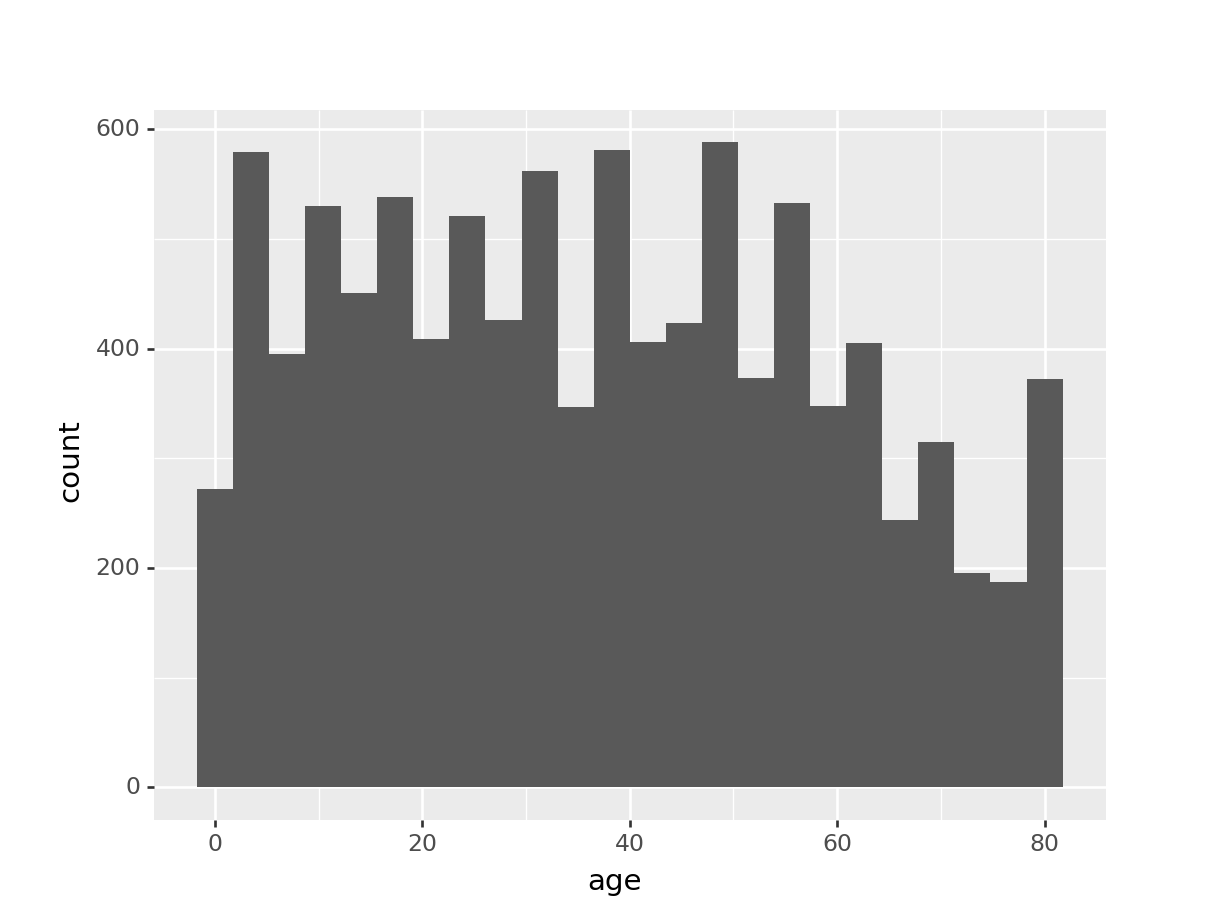
summary(nhanes_r$age) Min. 1st Qu. Median Mean 3rd Qu. Max.
0 17 36 37 54 80 histogram_age_r <- ggplot2::ggplot(nhanes_r, aes(x=age)) +
geom_histogram() +
theme_michaelmallari_r()
histogram_age_r
As with any numerical data (regardless of whether it’s discrete or continuous), we’re interested in knowing the summary statistics and visualize the distribution of the data.
Continuous
describe(nhanes_clean_jl.bmi)Summary Stats:
Length: 10000
Missing Count: 366
Mean: 26.660136
Minimum: 12.880000
1st Quartile: 21.580000
Median: 25.980000
3rd Quartile: 30.890000
Maximum: 81.250000
Type: Union{Missing, Float64}histogram_bmi_jl = Gadfly.plot(
nhanes_clean_jl,
x=:bmi,
Geom.histogram(bincount=83),
theme_michaelmallari_jl
);
nhanes_py["bmi"].describe()count 9634.000000
mean 26.660136
std 7.376579
min 12.880000
25% 21.580000
50% 25.980000
75% 30.890000
max 81.250000
Name: bmi, dtype: float64summary(nhanes_r$bmi) Min. 1st Qu. Median Mean 3rd Qu. Max. NA's
13 22 26 27 31 81 366 Qualitative or Categorical Data
Binary
CategoricalArrays.levels(nhanes_clean_jl.sleep_trouble)2-element Array{String3,1}:
"No"
"Yes"nhanes_jl[1:7, "sleep_trouble"]7-element PooledArrays.PooledArray{Union{Missing, String3},UInt32,1,Array{UInt32,1}}:
"Yes"
"Yes"
"Yes"
missing
"Yes"
missing
missingfrequency_table_simple_categorical_jl(nhanes_clean_jl, :sleep_trouble)3×4 DataFrame
Row │ sleep_trouble frequency percent_relative percent_cumulative
│ String3? Int64 Float64 Float64
─────┼────────────────────────────────────────────────────────────────
1 │ No 5799 57.99 57.99
2 │ missing 2228 22.28 80.27
3 │ Yes 1973 19.73 100.0nhanes_py.sleep_trouble.head(7)0 Yes
1 Yes
2 Yes
3 NaN
4 Yes
5 NaN
6 NaN
Name: sleep_trouble, dtype: objecthead(nhanes_r$sleep_trouble, 7)[1] TRUE TRUE TRUE FALSE TRUE FALSE FALSENominal
CategoricalArrays.levels(nhanes_clean_jl.sex_orientation)3-element Array{String15,1}:
"Bisexual"
"Heterosexual"
"Homosexual"nhanes_clean_jl[1:7, "sex_orientation"]7-element PooledArrays.PooledArray{Union{Missing, String15},UInt32,1,Array{UInt32,1}}:
"Heterosexual"
"Heterosexual"
"Heterosexual"
missing
"Heterosexual"
missing
missingfrequency_table_simple_categorical_jl(nhanes_clean_jl, :sex_orientation)4×4 DataFrame
Row │ sex_orientation frequency percent_relative percent_cumulative
│ String15? Int64 Float64 Float64
─────┼──────────────────────────────────────────────────────────────────
1 │ missing 5158 51.58 51.58
2 │ Heterosexual 4638 46.38 97.96
3 │ Bisexual 119 1.19 99.15
4 │ Homosexual 85 0.85 100.0# histogram_sex_orientation_jl = Gadfly.plot(
# nhanes_jl,
# x = :sex_orientation,
# Geom.histogram
# );nhanes_py.sex_orientation.head(7)0 Heterosexual
1 Heterosexual
2 Heterosexual
3 NaN
4 Heterosexual
5 NaN
6 NaN
Name: sex_orientation, dtype: objecthead(nhanes_r$work, 7)[1] NotWorking NotWorking NotWorking NotWorking
Levels: Looking NotWorking Workinghistogram_work_r <- ggplot2::ggplot(nhanes_r, aes(y=work)) +
geom_histogram(stat="count", colour=palette_michaelmallari_r[19], fill=palette_michaelmallari_r[19]) +
geom_text(
aes(label=..count..),
stat="count",
hjust=1.5,
colour=palette_michaelmallari_r[1]
) +
scale_y_discrete(limits=c("Working", "NotWorking", "NA", "Looking"), expand=c(0, 0), position="right") +
labs(
title="Employment Status",
alt="Employment Status",
subtitle="Frequency, n = 10,000",
x=NULL,
y=NULL,
caption="Data Source: https://www.cdc.gov/nchs/nhanes_r/"
) +
scale_y_discrete(expand=c(0, 0), position="right") +
theme_michaelmallari_r()
histogram_work_r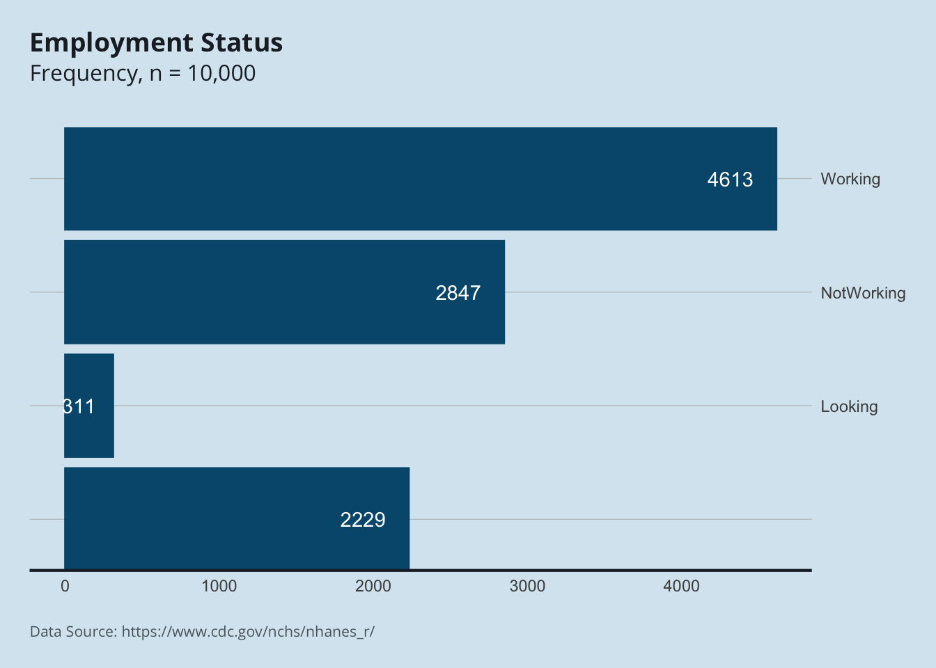
summary(nhanes_r$work) Looking NotWorking Working
2229 311 2847 4613 epiDisplay::tab1(nhanes_r$work, sort.group="decreasing", cum.percent=TRUE, graph=FALSE)nhanes_r$work :
Frequency Percent Cum. percent
Working 4613 46.1 46
NotWorking 2847 28.5 75
2229 22.3 97
Looking 311 3.1 100
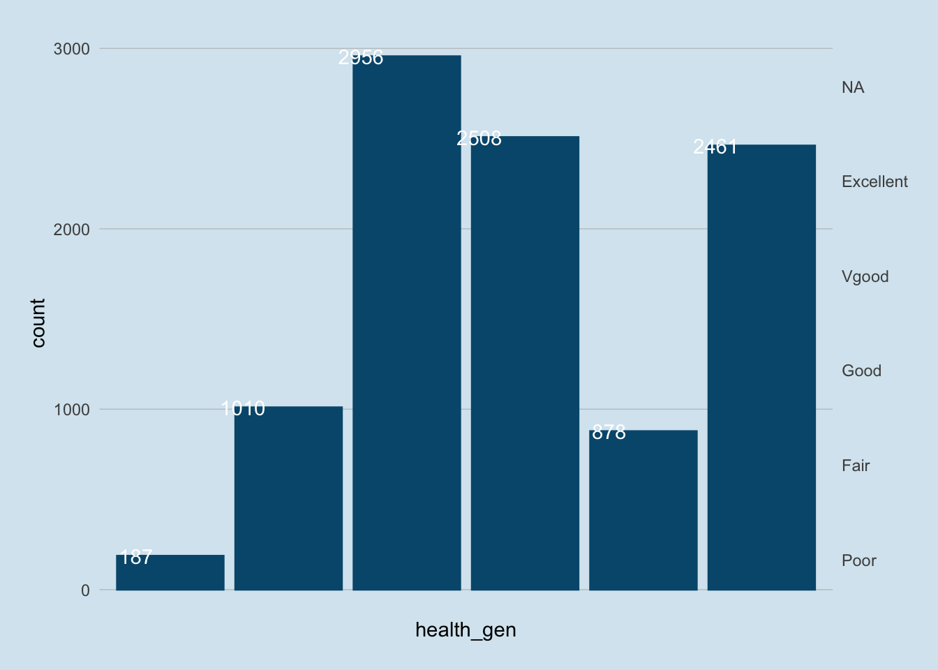
Total 10000 100.0 100Ordinal
CategoricalArrays.levels(nhanes_clean_jl.health_gen)5-element Array{String15,1}:
"Excellent"
"Fair"
"Good"
"Poor"
"Vgood"nhanes_clean_jl[1:7, "sex_orientation"]7-element PooledArrays.PooledArray{Union{Missing, String15},UInt32,1,Array{UInt32,1}}:
"Heterosexual"
"Heterosexual"
"Heterosexual"
missing
"Heterosexual"
missing
missingWe can see that this ordinal data (column or vector in the nhanes_clean_jl data frame) is not in the correct order. Setting the correct order is one of the common data wrangling tasks needed when working with ordinal data. Let’s set the correct order as Poor < Fair < Good < Vgood < Excellent.
nhanes_clean_jl.health_gen = CategoricalArrays.CategoricalArray{Union{Missing, String}}(nhanes_clean_jl.health_gen, ordered=true);
CategoricalArrays.levels!(nhanes_clean_jl.health_gen, ["Poor", "Fair", "Good", "Vgood", "Excellent"]);
CategoricalArrays.levels(nhanes_clean_jl.health_gen)
5-element Array{String,1}:
"Poor"
"Fair"
"Good"
"Vgood"
"Excellent"Now that the health_gen vector is in the correct order, it is now “clean” for data analyses, modeling, etc.
frequency_table_health_gen_jl = frequency_table_simple_categorical_jl(nhanes_clean_jl, :health_gen)6×4 DataFrame
Row │ health_gen frequency percent_relative percent_cumulative
│ Cat…? Int64 Float64 Float64
─────┼─────────────────────────────────────────────────────────────
1 │ Good 2956 29.56 29.56
2 │ Vgood 2508 25.08 54.64
3 │ missing 2461 24.61 79.25
4 │ Fair 1010 10.1 89.35
5 │ Excellent 878 8.78 98.13
6 │ Poor 187 1.87 100.0nhanes_py.loc[1:7, "health_gen"]1 Good
2 Good
3 NaN
4 Good
5 NaN
6 NaN
7 Vgood
Name: health_gen, dtype: category
Categories (5, object): ['Excellent', 'Fair', 'Good', 'Poor', 'Vgood']nhanes_r[1:7, "health_gen"][1] Good Good Good <NA> Good <NA> <NA>
Levels: Poor < Fair < Good < Vgood < Excellenthistogram_health_gen_r <- ggplot2::ggplot(nhanes_clean_r, aes(x=health_gen)) +
geom_histogram(stat="count", colour=palette_michaelmallari_r[19], fill=palette_michaelmallari_r[19]) +
geom_text(
aes(label=..count..),
stat="count",
hjust=1.5,
colour=palette_michaelmallari_r[1]
) +
scale_x_discrete(limits=rev(levels(nhanes_clean_r$health_gen)), expand=c(0, 0), position="right") +
scale_x_discrete(position="right") +
# labs(
# title="",
# alt="",
# subtitle="",
# x=NULL,
# y=NULL,
# caption="Data Source: https://www.kaggle.com/datasets/sveta151/tiktok-popular-songs-2019"
# ) +
theme_michaelmallari_r()
histogram_health_gen_r